Lab 5: Autocorrelation
Welcome to Lab 5!
Aim of the lab
In this guide you will learn how to:
- Access and use census data in R
- Run hypothesis tests
- Assess and visuralise autocorrelation
This lab guide follows and supplements the material presented in the textbook Spatial Autocorrelation in R.
This is a TWO WEEK LAB See here
for assignment guidelines. You must submit an .Rmd file and
its associated .html file.
Getting help
- Kiely (and often Dr G) will be present during your lab sessions. This
is the easiest way to get help.
- Dr G has weekly office hours and genuinely enjoys helping with R, even
if you feel stuck or overwhelmed.
- You may send a Canvas message to Kiely or Dr G (or if you are
completely lost).
Set-up. DON’T SKIP!
Create a project & get the data
There are two options here depending on whether you are using R-studio on the website (posit cloud) or your own computer (R-Desktop). If you are using a lab computer choose the R-Desktop route.
Option 1. Posit Cloud Website Users
Task 1. Create a project for Lab 5 (expand for instructions)
Task 2. Install more packages (expand for instructions)
Unfortunately on the website you need to install your packages each
time.
Go to to the packages tab, click install to get to the
app-store and download/install these packages:
readxlviridisggstatsplotterratigristidyversedplyrtmapelevatrosmdataggplot2ggthemesRColorBrewerplotlycols4allshinyjs
We will also need a package called sf, which runs a lot of the spatial commands in R. Unfortunately, posit cloud sometimes has a few technical issues with sf, so you will need to run a special command.
IN THE CONSOLE, run these two commands.
install.packages("remotes")
remotes::install_github(repo = "r-spatial/sf", ref = "93a25fd8e2f5c6af7c080f92141cb2b765a04a84")
T6_Packages.html
Reminder: Tutorial:
Packages cheatsheet.
Option 2. R-Desktop Users
Task 1. Create a project for Lab 5
Set-up your Lab 5 report
You are welcome to use/edit the template you made in previous labs. If you are unsure what I mean by that, follow these instructions.
Task. Create your RMarkdown file - expand & look at Tutorial 4B and 4C
Task. Edit your YAML code & ADD A NEW THEME
Lets use similar options to Lab 4. Remember YAML code is annoying to edit, because here, spaces really do matter. Everything has to be perfect or it won’t knit.
Select everything in my code chunk here and replace your YAML with this (remember the — on line 1 and at the end).
Now edit the author name to your own. If you wonder what Sys.Date() is, don’t touch it - it automatically gives you the current date.
Now change your theme to your favourite one of these - you can see what it looks like by pressing knit. Note, DO NOT put quote marks around the theme name.
- bootstrap
- cerulean
- cosmo
- darkly
- flatly
- journal
- lumen
- paper
- readable
- sandstone
- simplex
- spacelab
- united
- yeti
#---------------------------------------------------------
# NOTE, Your theme does NOT have quote marks around it
#---------------------------------------------------------
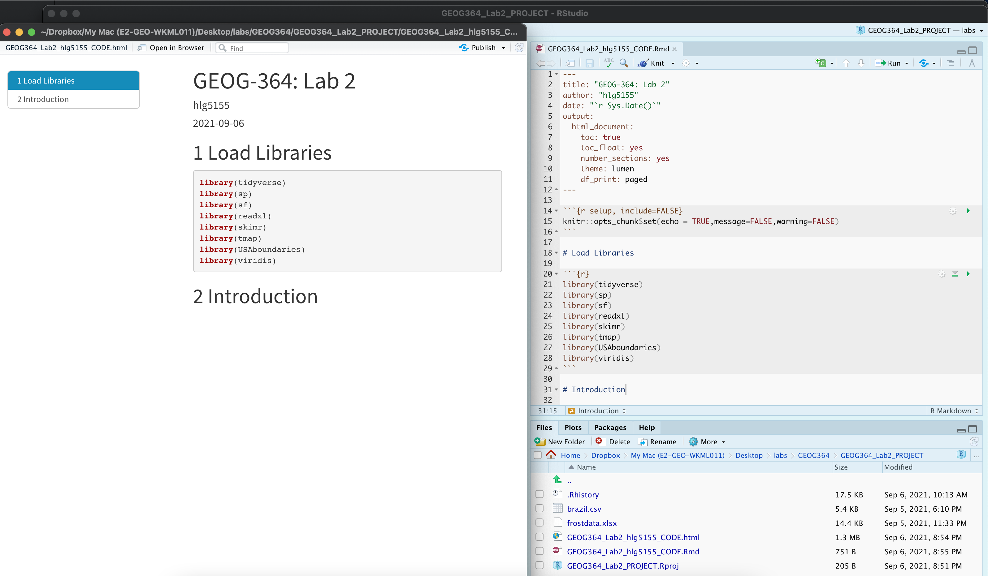
---
title: "GEOG-364 - Lab 5"
author: "hlg5155"
date: "`r Sys.Date()`"
output:
html_document:
toc: true
toc_float: yes
number_sections: yes
theme: lumen
df_print: paged
---Task. Delete the existing text and create/run your library code chunk
Click on your lab script (the Rmd file) and delete all the ‘welcome text’ after line 11.
Press enter a few times and make a new level-1 heading calledSet Up.We should have all the packages we need installed, but we need to open them. Make a new code chunk containing this code.
library(readxl)
library(tidyverse)
library(dplyr)
library(terra)
library(sf)
library(tmap)
library(elevatr)
library(osmdata)
library(ggstatsplot)
library(ggplot2)
library(ggthemes)
library(viridis)
library(RColorBrewer)
library(plotly)
library(units)
Press the green arrow on the right of the code chunk to run the code inside it. You will see a load of “loading text” telling your details about the packages you just loaded.
Press the green arrow AGAIN. The text should disappear unless there is an error.Note, remember to run this code chunk EVERY TIME your start R-Studio (in the same way you need to click on an app on your phone before you can use it).
You might need additional libraries as you work through the lab. If so, add them in this code chunk AND REMEMBER TO RERUN. If you see a little yellow bar at the top asking you to install them,click yes!
Task. Add warning=FALSE and message=FALSE to your library code chunk.
- Expand here for a tutorial.
Check your progress
Your lab script should now look similar this, but with your theme and YAML options of choice (you might have a few different libraries than in my screenshot). You should also be able to knit it successfully. If not, go back and do the previous sections!
Accessing US-Census Data
The tutorial below will show you how to download and use data from the US census and American Community survey. Read the lab instructions first, then us the tutorial to help you do it.
- Make a new section & explain ACS
Make a new section in your lab script called US-Census data
Using this page or google, read about the American Community Survey - https://www.census.gov/programs-surveys/acs/about.html
Now, Explain what the US-Census American Community survey is and why it’s a useful dataset. Make sure to include what the object of analysis is and its boundaries in time (e.g. does one survey represent all of US history?)
- Read through the tutorial below
As you read - know that, the tutorial is focused on Maine and New
Hampshire. YOU WILL BE FOCUSED ON IOWA. Looking at the list of
variables, choose one or two additional variables that interest you. For
example, past students have looked at water, poverty (access to
sanitation), access to broadband, demographics and crime etc.
Expand for tutorial - Census data
- Download census data using the tutorial.
Use the tutorial code to download county level American Community Survey for IOWA, including:
- housevalue (“B25075_001”)
- total_pop (“B05012_001”)
- total_house (“B25001_001”)
- med.income (“B19013_001”)
- AND a few variables of your own (see previous step)
REMEMBER THAT YOU NEED TO GET YOUR API KEY FIRST FROM THE START OF THE TUTORIAL, AND IT WON’T WORK UNTIL YOU HAVE FULLY RESTARTED R-STUDIO.
- Make 3 maps from this data that show something interesting about Iowa.
Write a few sentences under each one interpreting your results
e.g. look at google maps, why are certain counties/high or low.
Bonus marks for something that’s genuinely interesting, rather than just
two random variables you decided on.
If you want to continue to
improve your tmap chloropleths. https://rpubs.com/erikaaldisa/choroplethmapping
- The Modifiable Areal Map Problem MAUP
WE WILL COVER THIS ON WEDNESDAY Explain the modifiable areal map problem and both the shape and zone effects. Write any impacts of MAUP that you see in your analyses of Iowa and your reasoning.
- Chloropleths
Using google, explain what a chloropleth map is and why MAUP is a problem.
- Use the best practice for chloropleths
Look at the best practice for chloropleths https://blog.datawrapper.de/choroplethmaps/ and make a new version of one of your plots with at least one improvement, explaining what you did. If you can’t get it working, you can get most of the marks for explaining what you WANTED to do.
Moran’s I & Autocorrelation
Autocorrelation basics
Now we will focus on autocorrelation.
- Make a new section
Make a new section in your lab script called Autocorrelation. In this section, I will leave it up to you to make clear sub-headings to make it easy for grading.
- Explain in your report:
(see Monday’s lecture and reading)
- What is spatial autocorrelation and why is it important?
- What is positive/negative/zero autocorrelation and what patterns/processes would you expect to see.
- For one of the maps you made above, state which map you chose and explain whether you think you see positive/negative/zero autocorrelation (and your reasoning)
- Why will total population look much more clustered than population density?
Spatial weights matrices
To understand the autocorrelation, we first need to define neighbourhood.
- Read through the tutorial below
Expand for tutorial - Spatial weights
- Calculate the spatial weights
Now use the tutorial above to calculate and plot these neighbours and spatial weights matrix for your Iowa dataset. - QUEENS 1st order - ROOKS 2nd order
- Explain what you did
Below your code, briefly explain the difference between nearest neighbour, Rook’s, and Queen’s spatial weights matrices. Your answer should describe how each defines adjacency and what kinds of spatial relationships they capture.
- Are the Hawkeyes neighbours?
The Iowa Hawkeyes are based in Iowa City, Iowa (look up the county if needed). Your friend lives in Black Hawk County, Iowa. Using R code from the tutorial, determine whether Black Hawk County is a Rook’s 2nd-order neighbour of Iowa City’s county. Show your code and output.
Moran’s Scatterplots and Moran’s I
Now we have all the ingredients we can create a moran’s I scatterplot
- Read through the tutorial below ONLY up to the end of the scatterplot
Expand for tutorial - Moran’s scatter
- Create some plots
Use the code in the tutorial to create a Moran’s scatterplot for the median income in Iowa and your rook’s 1st order spatial weights matrix.
Moran’s hypothesis test
- Continue the tutorial
Expand for tutorial - Moran’s scatter
- Calculate Moran’s I
Calculate Moran’s I for the median income in Iowa and your rook’s 1st order spatial weights matrix.
- Run a hypothesis test
Calculate the results of Moran’s I hypothesis test for the median income in Iowa and your rook’s 1st order spatial weights matrix.
Interpret the answer fully in the text using the tutorial and lecture notes to help. Assume that I consider the answer to be significant at a p-value threshold of 0.01.
- Explain your answer
From your answer and the scatterplot, do you believe the field is positively negatively or zero(ly) autocorrelated? Explain your answer referring to the scatterplot.
Create a quick map of the median income in Iowa (you have the code for this higher in the lab!) and comment on your result compared to the map.
Advanced
Congratulations! If you have made it here you already have a
B.
For the next question, we will grade progressively depending
on how far through you get.
As always, an A grade is reasonable,
100% is hard.
OK, so you have now worked through an entire assessment of Moran’s I. For a given dataset, we have
- Read in the data
- Made it spatial and assigned a map projection
- (used things like st_make_value to remove features that crash the moran code)
- Calculated neighbours and spatial weights matrix of our choice
- Calculated the Moran’s I scatterplot and hypothesis test.
In the question below, I’m asking you to run the whole process for a new scenario. Remember you can copy your existing code into a single code chunk, like I did at the start of the tutorials.
- Try the full process (13 marks)
You already HAVE the code to do this You just need to copy/paste your code down here and edit for the new scenario.
Or see the beginning of each tutorial for a summary of the code. To make your life easier, look at the top of the page and you’ll see the tutorials in order. You’ll also find things like the census code for broadband access.
Create a new section called Advanced.
- For ‘broadband access’ for counties in Pennsylvania and 1st
order queens - 10 MARKS
- Download the data and wrangle
- Make a chloropleth map
- Calculate the moran’s I and show the moran’s scatterplot
- Run a hypothesis test & interpret, assuming I consider the result significant at p=0.05
- Relate everything back to the pattern you see and the PROCESSES creating broadband access patterns.
- Repeat for West Virginia and compare your results. Comment on any differences you see - 3 MARKS.
- SUPER-ADVANCED For the final 2 Marks
**You can easily get an A without attempting this.
In class we talked about calculating Moran’s I at differnet lags and there is a nice tutorial here. https://mgimond.github.io/Spatial/spatial-autocorrelation-in-r.html#app8_6
Using the tutorial, see if you can calculate the lagged Moran’s I for broadband access in PA.
Submitting your Lab
Remember to save your work throughout and to spell check your writing (next to the save button). Now, press the knit button again. If you have not made any mistakes in the code then R should create a html file in your lab3 folder, complete with a very recent time-stamp.
If you are on posit cloud:
You can download each of your .RmD and html files by:
Clicking on the little box next to the Rmd in the Files tab, then going to the little blue cogwheel (might need to make your Rstudio full screen) and clicking export.
Repeat the process exactly for the html file underneath it (e,g, just have the html clicked.)
Now go to Canvas and submit BOTH your html and your .Rmd file in Lab 5.
Posit desktop
Go to your Lab 5 folder, In that folder, double click on the html file. This will open it in your browser. CHECK THAT THIS IS WHAT YOU WANT TO SUBMIT
Now go to Canvas and submit BOTH your html and your .Rmd file in Lab 5.
CHECK THIS BEFORE YOU SUBMIT! (Lab)
People who use this section get better grades…
Grading rubric
- Submitting Rmd & HTML (15 pts)
- 20: Both .Rmd and .html submitted
- 10:Only one file submitted
- General style & writing (20 pts)
- 10: Great style:
You have written your answers below the relevant code chunk in full sentences in a way that is easy to find and grade. For example, you have written in full sentences, it is clear what your answers are referring to. You have used units where appropriate; no library-loading printouts; no code warnings; YAML works - 8: Minor issues:
Occasional hard-to-find answers; library-loading text printed; missing table of contents - 6: Major issues:
*Hard to find answers; multiple code issues
- 10: Great style:
US-Census Data - 20 MARKS
Download the census data & make/explain maps for Iowa [10]
Your MAUP answers [10]
Best practice [5]
Spatial weights matrix - 10 MARKS
You got the code working [5 MARKS]
Your answers / interpretation [5 MARKS]
Moran’s I & scatterplot - 10 MARKS
You got the code working [5 MARKS]
Your answers / interpretation [5 MARKS]
Morans Hypothesis test - 10 MARKS
You got the code working [5 MARKS]
Your answers / interpretation [5 MARKS]
Advanced - 13 MARKS
Sliding scale out of 10 for your code and interpretation of PA broadband [10]
Sliding scale out of 3 for your code and interpretation of West Virginia broadband [3]
Super advanced - 2 MARKS
You made a good effort [1]
Everything is working AND interpreted in the text [1]
Overall
Overall, here is what your lab should correspond to:
| Grade | % Mark | Rubric |
|---|---|---|
| A* | 98-100 | Exceptional. Not only was it near perfect, but the graders learned something. THIS IS HARD TO GET. |
| NA | 96+ | You went above and beyond |
| A | 93+: | Everything asked for with high quality. Class example |
| A- | 90+ | The odd minor mistake, All code done but not written up in full sentences etc. A little less care |
| B+ | 87+ | More minor mistakes. Things like missing units, getting the odd question wrong, no workings shown |
| B | 83+ | Solid work but the odd larger mistake or missing answer. Completely misinterpreted something, that type of thing |
| B- | 80+ | Starting to miss entire/questions sections, or multiple larger mistakes. Still a solid attempt. |
| C+ | 77+ | You made a good effort and did some things well, but there were a lot of problems. (e.g. you wrote up the text well, but messed up the code) |
| C | 70+ | It’s clear you tried and learned something. Just attending labs will get you this much as we can help you get to this stage |
| D | 60+ | You attempt the lab and submit something. Not clear you put in much effort or you had real issues |
| F | 0+ | Didn’t submit, or incredibly limited attempt. |
And.. finished!