Getting/Plotting US-Census data
R allows you to access and download all of the US Census and American Community survey data with a few quick commands.
These are two wonderful tutorials for using these functions in more depth.
All the code is summarised at the end in a single code chunk.
Libraries needed for this tutorial.
Make sure all of these libraries are at the top of your lab script in a code chunk, and run the code chunk! If you run the code chunk and it says a package is missing, either click “install” if the little yellow bar appears at the top, or go to the Packages tab, and click Install to go to the package ‘app store’.
library(readxl)
library(tidyverse)
library(dplyr)
library(terra)
library(sf)
library(tmap)
library(ggplot2)
library(ggthemes)
library(viridis)
library(RColorBrewer)
library(plotly)
library(spatstat)
library(sfdep)
library(tidycensus)
library(units)
Get an API/password
THIS IS A ONE OFF PROCESS. If you run the command several times or include it in your lab report, it will give an error and will not allow you to knit. Make sure that you run the command IN THE CONSOLE, not in a code chunk.
Sign up online
First, you need to sign up in advance for a password, called an API key. You can use Penn State as the organisation. In a few minutes, e-mail you a personal access code called an API key. Click the link in the e-mail to activate.
https://api.census.gov/data/key_signup.html
Sometimes your key will just stop working. If that happens, it’s fine to sign up for a new one.
Teach R your API key
You don’t need to type this password in every time you run R. Instead we will teach it to R once.
- IN THE CONSOLE!!,
Type this command, but replace “YOUR API KEY GOES HERE” with the password you were given. This will now save the password on your system.
# DO NOT RUN THIS IN A CODE CHUNK, COPY IT INTO THE CONSOLE & RUN IT THERE
tidycensus::census_api_key("YOUR API KEY GOES HERE", install=TRUE,overwrite=TRUE)

# Here is an imaginary example, YOU NEED YOUR OWN NUMBER
# census_api_key("d2a990g429206c51b54n98ec51886c6cf01a7ef2", install=TRUE,overwrite=TRUE)
FINALLY, RESTART R STUDIO OR NOTHING WILL
WORK!!
On your laptop, shut R-studio down and restart by going to your lab5
project and double clicking on the .RProj file. On the cloud, go to the
Session menu at the top and click “restart R and clear output”.
Downloading federal data using Get_ACS
TidyCensus allows you access to many large data-sets. For example
get_acs()Obtains data and feature geometry for the American Community Surveyget_decennial()Obtains data and feature geometry for the decennial US Censusget_estimates()Gets data from the US Census Bureau Population Estimates APIsget_flows()Obtains data and feature geometry for American Community Survey Migration Flows
Example
Each command has similar arguments. Here is an example for get_acs() where I download county level American Community Survey data for Maine and New Hampshire.
First, set up your code chunk carefully because it really likes to output spurious text. Add these code chunk options: {r, results=‘hide’,message=FALSE,warning=FALSE}
Here is the command.
# Download some data for Maine and NH using get_acs
# THIS WILL NOT WORK IF YOU DIDN'T RUN YOUR API KEY CODE & RESTART R-STUDIO

ACS_county.sf <- get_acs(geography = "county",
                         year = 2019,
                         variables = c(housevalue  = "B25075_001",  # house value
                                       total_pop   = "B05012_001",  # total population
                                       total_house = "B25001_001",  # no. houses
                                       med.income  = "B19013_001"), # median income
                         state = c("ME", "NH"),
                         survey = "acs5", geometry = TRUE,
                         output = "wide", show_call = FALSE)
Here is what each argument means:
geography: The level of geography we want the data in; in our case, the county. Other geographic options include “tract” for census tracts, plus tens more can be found here in the table https://walker-data.com/tidycensus/articles/basic-usage.htmlyear: The end year of the data.variables: The variables we want to bring in as specified in a vector you create using the function c(). Note that we created variable names of our own (e.g. “topop”) and we put the ACS IDs in quotes (“B03002_003”). Had we not done this, the variable names will come in as they are named in the ACS, which are not very descriptive.state: We can filter the counties to those in a specific state. Here it is c(“PA”, “NY”) for Pennsylvania and New York. If we don’t specify this, we get all counties in the United States - this is a HUGE download.survey: The specific Census survey were extracting data from. We want data from the 5-year American Community Survey, so we specify “acs5”. The ACS comes in 1-, 3-, and 5-year varieties.geometry: If geometry is set to FALSE, it just brings in a standard non-spatial table. If it’s set to true, it makes the data into a spatial sf file.wide: This makes on column for each variable, setting it to false would make one single column for all the estimates and one for the margin of error. We normally want wide=TRUE
How to find variable names
There are hundreds of variables you can download. You can see a full list here: https://www.socialexplorer.com/data/ACS2017_5yr/metadata/?ds=ACS17_5yr
For example:
- “B05012_001”, total population
- “B25001_001”, total housing units
- “B25075_001”, house value
- “B02001_004”, total who identify as native american
- “B03003_003”, total who identify as Hispanic
- “B03001_008”, total who identify as Hispanic Central A
- “B03001_016”, total who identify as Hispanic South A
- “B03002_003”, total who identify as white
- “B03002_004”, total who identify as black
- “B19013_001”, median income
- “B06010_011”, number of people making > 75000 USD
- “B05012_003”, number of foreign born people
- “B25035_001”, average house age
- “B25105_001”, monthly house expenditures
- “B25064_001”, median rent
- “B08101_049”, number who work from home
- “B25003_002”, total owner occupied
- “B25041_001”, total number of beds in the house
- “B28002_004”, total with broadband access
- “B25047_003”, total without plumbing
- “B25047_002”, all mobile homes -
- “B25024_010”, native mobile homes
- “B25032E_010”, total with complete plumbing
- “B15012_001” , total with at least a bachelors degree
If you add new variables, make sure they are inside the parentheses for the variable argument! A common error is to add them as a new line, not adding to the list of variables.
Wrangling census data
The ACS_county.sf object consists of an sf
vector layer representing census data aggregated at the county
subdivision level for 2019 (src. Census Bureau 5-year ACS).
If you got it working and click on/view ACS_county.sf from the Environment tab, you should now see that it has downloaded each one of your variables for every county in Maine and NH.
Estimates vs Margin of Error
In fact, for every one, it has downloaded the ESTIMATE of what they think that variable is for that region, but also has included the MARGIN-OF-ERROR, the 90% confidence interval on our result (90% of the time our result should be within this margin of error)
So any column-name with an E at the end is the estimate and anything with an M at the end are the error bars on that estimate.
e.g.
names(ACS_county.sf)## [1] "GEOID" "NAME" "housevalueE" "housevalueM" "total_popE"
## [6] "total_popM" "total_houseE" "total_houseM" "med.incomeE" "med.incomeM"
## [11] "geometry"Removing margin of error
To make your lives less confusing, we are going to remove the margin of error columns
# This is optional, for more advanced work, you probably want to keep the error columns

ACS_county.sf <- ACS_county.sf %>%
  select(
    GEOID,
    NAME,
    housevalue   = housevalueE,
    total_pop    = total_popE,
    total_house  = total_houseE,
    med.income   = med.incomeE,
    geometry
    )
Removing margin of error
Once we have the data, we want to do things with it.
# Change the map projection to Albers equal projection,
# then remove empty polygons (lakes etc) and fix any broken geometry
ACS_county.sf <- ACS_county.sf %>%
  st_transform(5070) %>%
  filter(!st_is_empty(geometry)) %>%
  st_make_valid()


# Find the areas in each county & change the units from metres squared to km squared
ACS_county.sf$Area  <- st_area(ACS_county.sf)
ACS_county.sf$Area  <- as.numeric(set_units(ACS_county.sf$Area,"km^2"))


# Divide the total population & housing by the area to give the population/housing density
ACS_county.sf$pop_density_km2  <- ACS_county.sf$total_pop   / ACS_county.sf$Area
ACS_county.sf$house_density_km2 <- ACS_county.sf$total_house / ACS_county.sf$Area

# And tidy up
ACS_county.sf <- st_make_valid(ACS_county.sf)
Plotting census data using tm_polygons
THIS IS AN EXAMPLE.
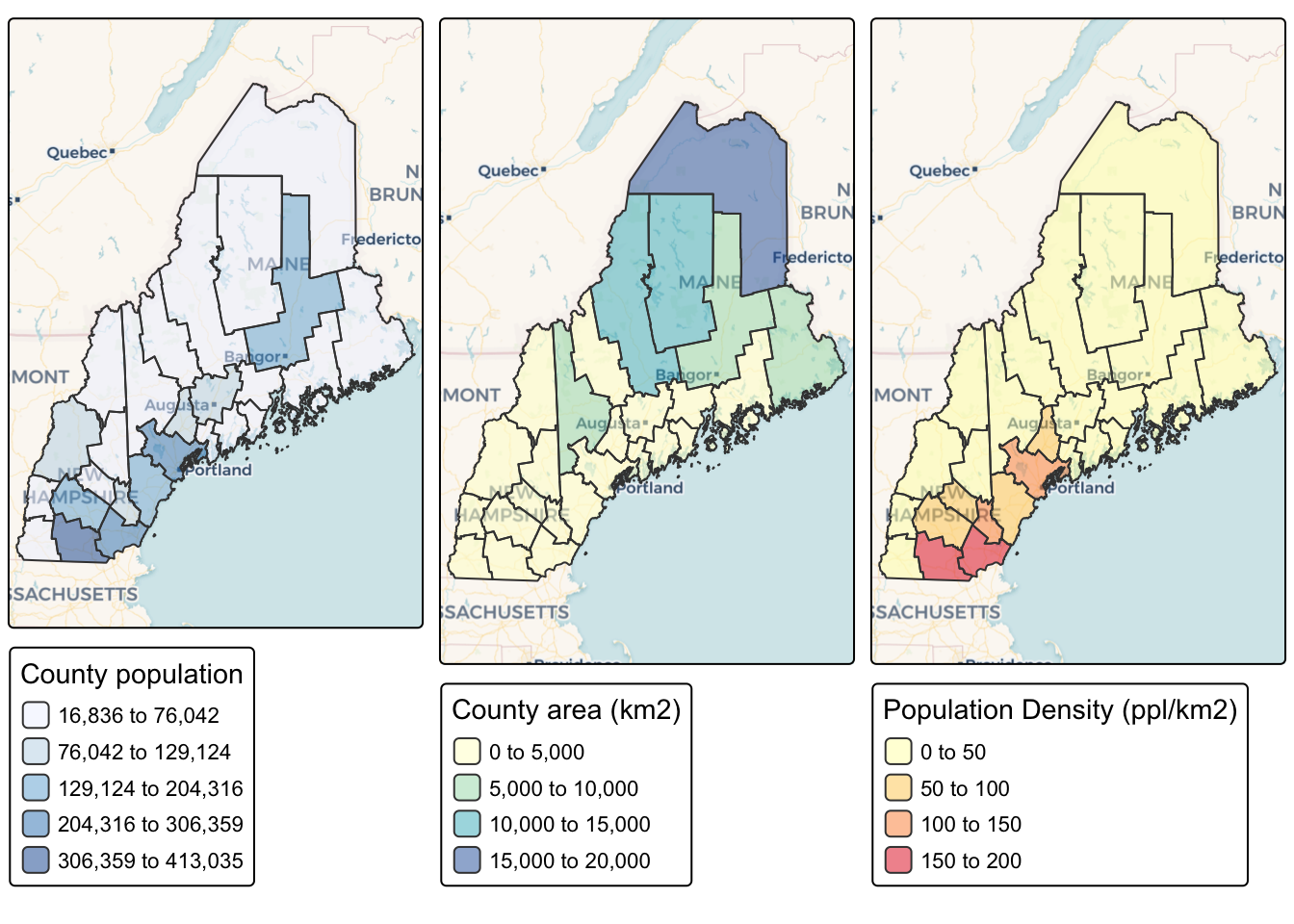
You can now plot the census data like any other spatial dataset. For example, here is how to plot three things together. Again, I suggest including message=FALSE and warning=FALSE in your code chunk options.
For other color options, type & run cols4all::c4a_palettes() INTO THE CONSOLE.
# I make each map but save them rather than show them on the screen

# Total population
map_totalpop <- tm_shape(ACS_county.sf) +
                  tm_polygons(fill = "total_pop",
                     fill.scale  = tm_scale_intervals(
                                     values = "brewer.blues",
                                     style = "jenks"),
                     fill_alpha  = 0.5,
                     fill.legend = tm_legend("County population")) +
                tm_basemap("CartoDB.Voyager")

# Area
map_area <- tm_shape(ACS_county.sf) +
                  tm_polygons(fill = "Area",
                     fill.scale  = tm_scale_intervals(
                                     values = "brewer.yl_gn_bu",
                                     style. = "pretty"),
                     fill_alpha  = 0.5,
                     fill.legend = tm_legend("County area (km2)")) +
                tm_basemap("CartoDB.Voyager")


map_popdens <- tm_shape(ACS_county.sf) +
                  tm_polygons(fill = "pop_density_km2",
                     fill.scale  = tm_scale_intervals(
                                     values = "brewer.yl_or_rd",
                                     style. = "jenks"),
                     fill_alpha  = 0.5,
                     fill.legend = tm_legend("Population Density (ppl/km2)")) +
                tm_basemap("CartoDB.Voyager")


# Now show them together
tmap_mode("plot")
tmap_arrange(map_totalpop,map_area,map_popdens)
There are a load more ideas here for making pretty tmap plots: - http://zevross.com/blog/2018/10/02/creating-beautiful-demographic-maps-in-r-with-the-tidycensus-and-tmap-packages/
Code summary
library(readxl)
library(tidyverse)
library(dplyr)
library(terra)
library(sf)
library(tmap)
library(ggplot2)
library(ggthemes)
library(viridis)
library(RColorBrewer)
library(plotly)
library(spatstat)
library(sfdep)
library(tidycensus)


# Download some data for Maine and NH using get_acs
# THIS WILL NOT WORK IF YOU DID'T RUN YOUR API KEY CODE & RESTART R-STUDIO
ACS_county.sf <- get_acs(geography = "county",
                         year = 2019,
                         variables = c(housevalue  = "B25075_001",  # house value
                                       total_pop   = "B05012_001",  # total population
                                       total_house = "B25001_001",  # no. houses
                                       med.income  = "B19013_001"), # median income
                         state = c("ME", "NH"),
                         survey = "acs5", geometry = TRUE,
                         output = "wide", show_call = FALSE)
## | | | 0% | | | 1% | |= | 1% | |= | 2% | |== | 2% | |== | 3% | |== | 4% | |=== | 4% | |=== | 5% | |==== | 5% | |==== | 6% | |===== | 7% | |===== | 8% | |====== | 8% | |====== | 9% | |======= | 9% | |======= | 10% | |======= | 11% | |======== | 11% | |======== | 12% | |========= | 12% | |========= | 13% | |========= | 14% | |========== | 14% | |========== | 15% | |=========== | 15% | |=========== | 16% | |============ | 17% | |============ | 18% | |============= | 18% | |============= | 19% | |============== | 19% | |============== | 20% | |============== | 21% | |=============== | 21% | |=============== | 22% | |================ | 22% | |================ | 23% | |================ | 24% | |================= | 24% | |================= | 25% | |================== | 25% | |================== | 26% | |=================== | 26% | |=================== | 27% | |=================== | 28% | |==================== | 28% | |==================== | 29% | |===================== | 29% | |===================== | 30% | |===================== | 31% | |====================== | 31% | |====================== | 32% | |======================= | 32% | |======================= | 33% | |======================== | 34% | |======================== | 35% | |========================= | 35% | |========================= | 36% | |========================== | 36% | |========================== | 37% | |========================== | 38% | |=========================== | 38% | |=========================== | 39% | |============================ | 39% | |============================ | 40% | |============================ | 41% | |============================= | 41% | |============================= | 42% | |============================== | 42% | |============================== | 43% | |=============================== | 44% | |=============================== | 45% | |================================ | 45% | |================================ | 46% | |================================= | 46% | |================================= | 47% | |================================= | 48% | |================================== | 48% | |================================== | 49% | |=================================== | 49% | |=================================== | 50% | |=================================== | 51% | |==================================== | 51% | |==================================== | 52% | |===================================== | 52% | |===================================== | 53% | |====================================== | 54% | |====================================== | 55% | |======================================= | 55% | |======================================= | 56% | |======================================== | 56% | |======================================== | 57% | |======================================== | 58% | |========================================= | 58% | |========================================= | 59% | |========================================== | 59% | |========================================== | 60% | |========================================== | 61% | |=========================================== | 61% | |=========================================== | 62% | |============================================ | 62% | |============================================ | 63% | |============================================ | 64% | |============================================= | 64% | |============================================= | 65% | |============================================== | 65% | |============================================== | 66% | |=============================================== | 67% | |=============================================== | 68% | |================================================ | 68% | |================================================ | 69% | |================================================= | 69% | |================================================= | 70% | |================================================= | 71% | |================================================== | 71% | |================================================== | 72% | |=================================================== | 72% | |=================================================== | 73% | |=================================================== | 74% | |==================================================== | 74% | |==================================================== | 75% | |===================================================== | 75% | |===================================================== | 76% | |====================================================== | 77% | |====================================================== | 78% | |======================================================= | 78% | |======================================================= | 79% | |======================================================== | 79% | |======================================================== | 80% | |======================================================== | 81% | |========================================================= | 81% | |========================================================= | 82% | |========================================================== | 82% | |========================================================== | 83% | |========================================================== | 84% | |=========================================================== | 84% | |=========================================================== | 85% | |============================================================ | 85% | |============================================================ | 86% | |============================================================= | 86% | |============================================================= | 87% | |============================================================= | 88% | |============================================================== | 88% | |============================================================== | 89% | |=============================================================== | 89% | |=============================================================== | 90% | |=============================================================== | 91% | |================================================================ | 91% | |================================================================ | 92% | |================================================================= | 92% | |================================================================= | 93% | |================================================================== | 94% | |================================================================== | 95% | |=================================================================== | 95% | |=================================================================== | 96% | |==================================================================== | 96% | |==================================================================== | 97% | |==================================================================== | 98% | |===================================================================== | 98% | |===================================================================== | 99% | |======================================================================| 99% | |======================================================================| 100%# OPTIONAL. For more advanced work, you probably want to keep the error columns
# If you don't run it, remember all your columns have an E on the end of the name
ACS_county.sf <- ACS_county.sf %>%
select(
GEOID,
NAME,
housevalue = housevalueE,
total_pop = total_popE,
total_house = total_houseE,
med.income = med.incomeE,
geometry
)
# Change the map projection to Albers equal projection,
# then remove empty polygons (lakes etc) and fix any broken geometry
ACS_county.sf <- ACS_county.sf %>%
st_transform(5070) %>%
filter(!st_is_empty(geometry)) %>%
st_make_valid()
# Find the areas in each county & change the units from metres squared to km squared
ACS_county.sf$Area <- st_area(ACS_county.sf)
ACS_county.sf$Area <- as.numeric(set_units(ACS_county.sf$Area,"km^2"))
# OPTIONAL & DEPENDS ON THE VARIABLES YOU DOWNLOAD
# Divide the total population & housing by the area to give the population/housing density
ACS_county.sf$pop_density_km2 <- ACS_county.sf$total_pop / ACS_county.sf$Area
ACS_county.sf$house_density_km2 <- ACS_county.sf$total_house / ACS_county.sf$Area
# OPTIONAL, YOU DON'T HAVE TO DO THIS
# Example plots
# Total population
map_totalpop <- tm_shape(ACS_county.sf) +
tm_polygons(fill = "total_pop",
fill.scale = tm_scale_intervals(
values = "brewer.blues",
style = "jenks"),
fill_alpha = 0.5,
fill.legend = tm_legend("County population")) +
tm_basemap("CartoDB.Voyager")
# Area
map_area <- tm_shape(ACS_county.sf) +
tm_polygons(fill = "Area",
fill.scale = tm_scale_intervals(
values = "brewer.yl_gn_bu",
style. = "pretty"),
fill_alpha = 0.5,
fill.legend = tm_legend("County area (km2)")) +
tm_basemap("CartoDB.Voyager")
map_popdens <- tm_shape(ACS_county.sf) +
tm_polygons(fill = "pop_density_km2",
fill.scale = tm_scale_intervals(
values = "brewer.yl_or_rd",
style. = "jenks"),
fill_alpha = 0.5,
fill.legend = tm_legend("Population Density (ppl/km2)")) +
tm_basemap("CartoDB.Voyager")
# Now show them together
tmap_mode("plot")
tmap_arrange(map_totalpop,map_area,map_popdens)