Lab 6: LISA and Regression
Welcome to Lab 6!
Aim of the lab
In this guide you will learn how to:
- Run LISA analyses
- Run a regression analysis and look at spatial residuals
This is a TWO WEEK LAB See here
for assignment guidelines. You must submit an .Rmd file and
its associated .html file.
Getting help
- Kiely (and often Dr G) will be present during your lab sessions. This
is the easiest way to get help.
- Dr G has weekly office hours and genuinely enjoys helping with R, even
if you feel stuck or overwhelmed.
- You may send a Canvas message to Kiely or Dr G (or if you are
completely lost).
Set-up. DON’T SKIP!
Create a project & get the data
There are two options here depending on whether you are using R-studio on the website (posit cloud) or your own computer (R-Desktop). If you are using a lab computer choose the R-Desktop route.
Option 1. Posit Cloud Website Users
Task 1. Create a project for Lab 6 (expand for instructions)
Task 2. Install more packages (expand for instructions)
Unfortunately on the website you need to install your packages each
time.
Go to to the packages tab, click install to get to the
app-store and download/install these packages:
readxlviridisggstatsplotterratigristidyversedplyrtmapelevatrosmdataggplot2ggthemesRColorBrewerplotlycols4allshinyjs
We will also need a package called sf, which runs a lot of the spatial commands in R. Unfortunately, posit cloud sometimes has a few technical issues with sf, so you will need to run a special command.
IN THE CONSOLE, run these two commands.
install.packages("remotes")
remotes::install_github(repo = "r-spatial/sf", ref = "93a25fd8e2f5c6af7c080f92141cb2b765a04a84")
T6_Packages.html
Reminder: Tutorial:
Packages cheatsheet.
Option 2. R-Desktop Users
Task 1. Create a project for Lab 6
Set-up your Lab 6 report
You are welcome to use/edit the template you made in previous labs. If you are unsure what I mean by that, follow these instructions.
Task. Create your RMarkdown file - expand & look at Tutorial 4B and 4C
Task. Edit your YAML code & ADD A NEW THEME
Lets use similar options to Lab 4. Remember YAML code is annoying to edit, because here, spaces really do matter. Everything has to be perfect or it won’t knit.
Select everything in my code chunk here and replace your YAML with this (remember the — on line 1 and at the end).
Now edit the author name to your own. If you wonder what Sys.Date() is, don’t touch it - it automatically gives you the current date.
Now change your theme to your favourite one of these - you can see what it looks like by pressing knit. Note, DO NOT put quote marks around the theme name.
- bootstrap
- cerulean
- cosmo
- darkly
- flatly
- journal
- lumen
- paper
- readable
- sandstone
- simplex
- spacelab
- united
- yeti
#---------------------------------------------------------
# NOTE, Your theme does NOT have quote marks around it
#---------------------------------------------------------
---
title: "GEOG-364 - Lab 6"
author: "hlg5155"
date: "`r Sys.Date()`"
output:
  html_document:
    toc: true
    toc_float: yes
    number_sections: yes
    theme: lumen
    df_print: paged
---
Task. Delete the existing text and create/run your library code chunk
Click on your lab script (the Rmd file) and delete all the ‘welcome text’ after line 11.
Press enter a few times and make a new level-1 heading calledSet Up.We should have all the packages we need installed, but we need to open them. Make a new code chunk containing this code.
library(readxl)
library(tidyverse)
library(dplyr)
library(terra)
library(sf)
library(tmap)
library(elevatr)
library(osmdata)
library(ggstatsplot)
library(ggplot2)
library(ggthemes)
library(viridis)
library(RColorBrewer)
library(plotly)
library(units)
Press the green arrow on the right of the code chunk to run the code inside it. You will see a load of “loading text” telling your details about the packages you just loaded.
Press the green arrow AGAIN. The text should disappear unless there is an error.Note, remember to run this code chunk EVERY TIME your start R-Studio (in the same way you need to click on an app on your phone before you can use it).
You might need additional libraries as you work through the lab. If so, add them in this code chunk AND REMEMBER TO RERUN. If you see a little yellow bar at the top asking you to install them,click yes!
Task. Add warning=FALSE and message=FALSE to your library code chunk.
Check your progress
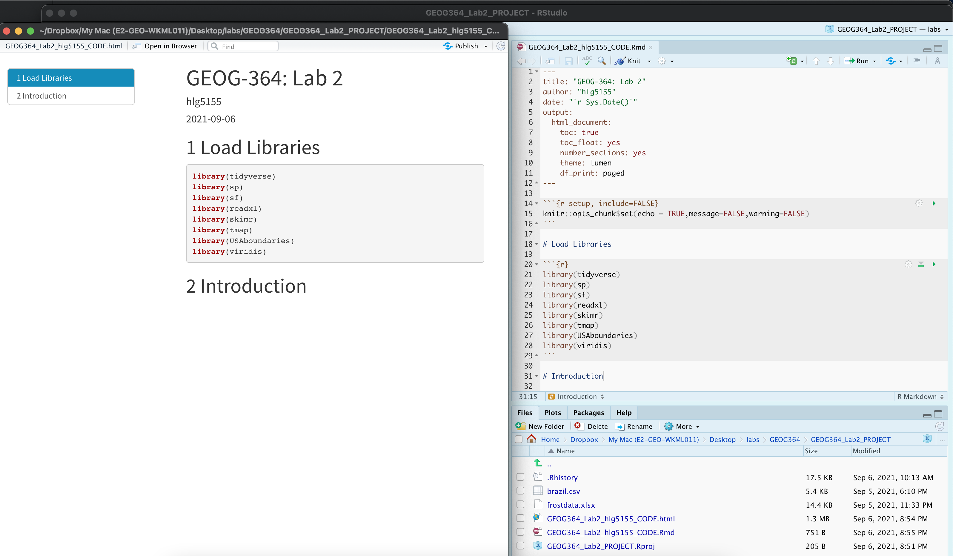
Your lab script should now look similar this, but with your theme and YAML options of choice (you might have a few different libraries than in my screenshot). You should also be able to knit it successfully. If not, go back and do the previous sections!
WEEK 1
This week we will try a new approach. I will work through a tutorial on local autocorrelation using one dataset. Please create a new, separate Rmd file for the tutorial. Do not work in your lab script for this part, and do not submit the tutorial file. Follow along and make sure it knits.
After the tutorial, you will complete a similar analysis on a different dataset in your actual lab script, using the questions below.
You should not submit the tutorial file. Creating one simply lets you follow along and copy code into your main lab script later. Only the work in your lab script will be submitted and assessed. We will DEDUCT MARKS for submitting anything about Chicago/the tutorial
A. Getting the data
- Look at the tutorial
Run through STEP 1 of the tutorial here https://psu-spatial.github.io/Geog364-2025/Tutorial_LISA.html You should stop when you made maps of the city. e.g. don’t carry onto step 2.
- Create your own,
Now, IN YOUR LAB SCRIPT, reproduce the tutorial for any largish city of your choice in the USA.
Get the code working and making the plots.
For each step, in your own words explain what you are doing for each piece of code and why you chose your city.
If you get errors, choose a different city!
B. Global Autocorrelation
- Look at STEP 2 of the tutorial
Run through STEP 2 of the tutorial here https://psu-spatial.github.io/Geog364-2025/Tutorial_LISA.html. Don’t carry onto Local Moran’s I.
- Create your own,
Now, continue for your city:
Creating a single spatial weights matrix of your choice (e.g. you could use EITHER queens/rooks/nearest neighbour or anything else)
Then run a Moran’s scatterplot and Moran’s test.
In the text, fully write out the hypothesis test for your city (you can choose the alternative hypothesis)
In the text, describe the pattern you see in the moran’s scatterplot and relate to your map.
C. Autocorrelation LISA
- Look at STEP 3 of the tutorial
Run through the rest of STEP 3 of the tutorial here https://psu-spatial.github.io/Geog364-2025/Tutorial_LISA.html .
- Create your own.
Now make some LISA plots for your city. We will discuss what these mean during Wednesdays class.
- Interpret your results in the text.
Based on that, see if you can interpret the results for your city in your lab report. Remember you can change your background map to identify where places are and do some googling! Your answer should talk about
What your results mean (e.g. what are the colors and how do they correspond to your variable)
The significance of your results e.g. where is highly significant and where is not?
Whether your results correspond to reality.
For example- Is your “high surrounded by high” downtown? rich suburbs?
- Is your “low surrounded by low” poorer areas?
- Any outliers and can you work out WHY they are outliers
WEEK 2
D. Update your data
To make your regression example more interesting, let’s update your data input.
- Update data
- Scroll to the top of your lab report, where you download the census data. E.g. it will look something like this but for your city
IL.Census.sf <- get_acs(geography = "tract",
                year = 2017,
                variables = c(total_pop   = "B05012_001", # total population
                              income.gt75 = "B06010_011"), # people making > 75000 USD
                state = "IL",
                survey = "acs5",
                geometry = TRUE,
                output="wide",
cache_table = TRUE)- Edit your code to add in these additional variables and re-run (I just copied in the missing lines leaving the rest identical)
IL.Census.sf <- get_acs(
   geography = "tract",
   year = 2017,
   variables = c(
      total_pop        = "B05012_001", # total population
      total_house      = "B25001_001", #total housing units
      income.gt75      = "B06010_011",# number of people making > 75000 USD
      med.income       = "B19013_001", #median income
      total.foreignppl = "B05012_003", #number of foreign born people
      total.BAdegree   = "B15012_001" , #total with at least a bachelors degree
      total.workhome   = "B08101_049", #number who work from home#total housing units
      house.mean_age   = "B25035_001", #average house age
      house.mean_beds  = "B25041_001", #total homes number of beds in the house
      housetotal.owneroccupied = "B25003_002", #total homes owner occupied
      housetotal.broadband  = "B28002_004"), #total homes with broadband access
   state = "IL",
   survey = "acs5",
   geometry = TRUE,
   output = "wide",
cache_table = TRUE)- Now scroll down to where you selected the variable names. It should look like this but for your city
# Remove and rename error columns
IL.Census.sf <- IL.Census.sf %>%
  dplyr::select(
    GEOID,
    NAME,
    total_pop    = total_popE,
    income.gt75  = income.gt75E,
geometry )- Edit so it looks like this for your city.
# Remove and rename error columns
IL.Census.sf <- IL.Census.sf %>%
   dplyr::select(
      GEOID,
      NAME,
      total_pop        = total_popE,
      total_house      = total_houseE,
      income.gt75      = income.gt75E,
      med.income       = med.incomeE,
      total.foreignppl = total.foreignpplE,
      total.BAdegree   = total.BAdegreeE,
      total.workhome   = total.workhomeE,
      house.mean_age   = house.mean_ageE,
      house.mean_beds  = house.mean_bedsE,
      housetotal.owneroccupied = housetotal.owneroccupiedE,
      housetotal.broadband     = housetotal.broadbandE,
geometry )- Now find the bit that looks like this where you calculate the densities
IL.Census.sf$pop.density_km2  <- IL.Census.sf$total_pop   / IL.Census.sf$Area
IL.Census.sf$percent.income.gt75 <- IL.Census.sf$income.gt75 / IL.Census.sf$total_pop- and edit so it looks like this for your city.
IL.Census.sf <- IL.Census.sf %>%
  mutate(
    pop.density_km2    = total_pop   / Area,
    house.density_km2  = total_house / Area,
    percent.income.gt75 = income.gt75 / total_pop,
    percent.foreignppl = total.foreignppl / total_pop,
    percent.BAdegree   = total.BAdegree   / total_pop,
    percent.workhome   = total.workhome   / total_pop,
    housepercent.owneroccupied = housetotal.owneroccupied / total_house,
    housepercent.broadband     = housetotal.broadband     / total_house  )
WHY DID I ASK YOU TO DO THIS?
The reason I’m asking you to update your code rather than re-download
fresh data is that this mirrors how real data analysis works. When
something in your project changes—especially your input data—it’s
important to adjust your existing script and run it cleanly from the
top. This ensures that your workflow is reproducible and that every
result in your lab comes from the same code, with no hidden steps or
leftover objects from earlier runs. It also prevents accidental copies
of the data, mismatched versions, or silent mistakes that can happen
when you download things manually.
This habit will matter more and more as your projects get larger: a careful, repeatable workflow is one of the most valuable skills you can build in R.
E. Finding a predictor
- Look at the tutorial
Run through STEP 1 of the tutorial here https://psu-spatial.github.io/Geog364-2025/Tutorial_Regression.html You should stop when you made maps of the city. e.g. don’t carry onto step 2.
- Create your own,
Now, IN YOUR LAB SCRIPT, get it working for your city.
Get the code working and making the plots.
Then look at all your potential predictors and decide which one you want to use to predict the percentage of people making > 75K in your city
Remember to write up your object, population etc and tell me if you removed any outliers.
If you get errors, tell Kiely immediately! (or try a different variable)
F. Regression model
- Look at the tutorial
Run through STEP 2 of the tutorial here https://psu-spatial.github.io/Geog364-2025/Tutorial_Regression.html Don’t carry onto step 3.
- Create your own,
Now, IN YOUR LAB SCRIPT, choose the predictor that best predicts your response variable
Run a regression model using lm
Write out the equation using latex, interpret the slope and intercept in the text
Add a new scatterplot including the line of best fit (no error bars e.g. use the tutorial version)
G. Mapping results
- Look at the tutorial
Run through STEP 3 of the tutorial here https://psu-spatial.github.io/Geog364-2025/Tutorial_Regression.html Don’t carry onto step 4.
- Create your own,
Now, IN YOUR LAB SCRIPT,
Make a maps of your response variable, predicted response and residuals. Make the style your own.
Discuss what you see in the text & interpret how good the model is in your opinion.
H. Spatial residuals
- Look at the tutorial
Run through STEP 4 of the tutorial here https://psu-spatial.github.io/Geog364-2025/Tutorial_Regression.html
- Create your own for your city
Now, IN YOUR LAB SCRIPT,
Make a Moran’s Scatterplot of your residuals and interpret what you see in the text
Run a full two sided moran’s hypothesis test on your residuals and write out everything in the text
Run a LISA analysis on your residuals and interpret in the text.
I. Lab Summary
- Reflection
Finally, imagine you are helping with some some analysis for your chosen city’s council. Explain in clear language what you have found for:
The autocorrelation & patterns in population density
The spatial pattern of people making more than $75K and links to the underlying processes for your particular city/geography.
What variables show promise in predicting the number of people making more than $75K
Whether your model meets the requirement of spatial independence and if there are any spatial patterns that are particularly interesting in the residuals.
Finally, if you could add a SECOND variable to account for some of the remaining spatial variability, what would you choose (either in the list you downloaded or more widely).
- Tidy up your report
Now go back and tidy up your report.
Add headings, subheadings etc so it’s easy for us to find all your answers.
Check everything has units included
Make sure your code isn’t printing out loads and loads of spurious numbers/text, You don’t have to include every line of code you wrote.
Make sure everything in your lab is linked to YOUR city. Any tutorial/Chicago examples should be separate (and you don’t need to submit thm)
Submitting your Lab
Remember to save your work throughout and to spell check your writing (next to the save button). Now, press the knit button again. If you have not made any mistakes in the code then R should create a html file in your lab3 folder, complete with a very recent time-stamp.
If you are on posit cloud:
You can download each of your .RmD and html files by:
Clicking on the little box next to the Rmd in the Files tab, then going to the little blue cogwheel (might need to make your Rstudio full screen) and clicking export.
Repeat the process exactly for the html file underneath it (e,g, just have the html clicked.)
Now go to Canvas and submit BOTH your html and your .Rmd file in Lab 6.
Posit desktop
Go to your Lab 6 folder, In that folder, double click on the html file. This will open it in your browser. CHECK THAT THIS IS WHAT YOU WANT TO SUBMIT
Now go to Canvas and submit BOTH your html and your .Rmd file in Lab 6.
GRADING RUBRIC
To come
Overall
Overall, here is what your lab should correspond to:
| Grade | % Mark | Rubric |
|---|---|---|
| A* | 98-100 | Exceptional. Not only was it near perfect, but the graders learned something. THIS IS HARD TO GET. |
| NA | 96+ | You went above and beyond |
| A | 93+: | Everything asked for with high quality. Class example |
| A- | 90+ | The odd minor mistake, All code done but not written up in full sentences etc. A little less care |
| B+ | 87+ | More minor mistakes. Things like missing units, getting the odd question wrong, no workings shown |
| B | 83+ | Solid work but the odd larger mistake or missing answer. Completely misinterpreted something, that type of thing |
| B- | 80+ | Starting to miss entire/questions sections, or multiple larger mistakes. Still a solid attempt. |
| C+ | 77+ | You made a good effort and did some things well, but there were a lot of problems. (e.g. you wrote up the text well, but messed up the code) |
| C | 70+ | It’s clear you tried and learned something. Just attending labs will get you this much as we can help you get to this stage |
| D | 60+ | You attempt the lab and submit something. Not clear you put in much effort or you had real issues |
| F | 0+ | Didn’t submit, or incredibly limited attempt. |
And.. finished!