T10: Regression

Regression models

Now we will fit our first regression model.

“Standard” regression output

The command to do this is lm() e.g. linear model.

output <- lm(y_column ~ x_column,data=tablename)
output

NOTE, THE WEIRD ~ SYMBOL. This means “depends on” and it’s how we tell R what the response variable is. E.g. y depends on x, or y=mx+c.

For example for the NYHouses data, it would be

# response = Price, predictor = Lot size
Model1.lm <- lm(Price ~ Lot,data=HousesNY)
Model1.lm

Call:
lm(formula = Price ~ Lot, data = HousesNY)

Coefficients:
(Intercept)          Lot  
   114.0911      -0.5749  

So we are saying here that the equation is

Expected_Average_Price = -0.5749*Lot_Size + 114.0911

E.g. the average expected price house with no Lot/Garden is 114.09

Printing out the equation

You can also directly get the code for the model equation by the equatiomatic package

# YOU MIGHT NEED TO INSTALL THIS PACKAGE (SEE THE TUTORIAL)
library(equatiomatic)
extract_eq(Model1.lm,use_coefs=FALSE)

To make it print out directly, put “asis=TRUE” as a code chunk option e.g. this code

See the asis in the top, this prints the output directly when you knit

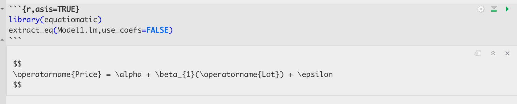
Turns into this:

library(equatiomatic)
extract_eq(Model1.lm,use_coefs=FALSE)

\[ \operatorname{Price} = \alpha + \beta_{1}(\operatorname{Lot}) + \epsilon \]

You can also look at the summary by looking at the summary command:

summary(Model1.lm)

Call:
lm(formula = Price ~ Lot, data = HousesNY)

Residuals:
    Min      1Q  Median      3Q     Max 
-74.775 -30.201  -5.941  27.070  83.984 

Coefficients:
            Estimate Std. Error t value Pr(>|t|)    
(Intercept) 114.0911     8.3639  13.641   <2e-16 ***
Lot          -0.5749     7.6113  -0.076     0.94    
---
Signif. codes:  0 '***' 0.001 '**' 0.01 '*' 0.05 '.' 0.1 ' ' 1

Residual standard error: 41.83 on 51 degrees of freedom
Multiple R-squared:  0.0001119, Adjusted R-squared:  -0.01949 
F-statistic: 0.005705 on 1 and 51 DF,  p-value: 0.9401

In both cases, we have an estimate of the intercept (0.6386) and of the gradient (-13.8103). We will discuss the other values in later labs/lectures.

Now let’s see how to add the regression line to our scatterplot. We can do this using abline(REGRESSION_VARIABLE), where regression_variable is the name of the variable you saved the output of lm to. For example.

plot(HousesNY$Price ~ HousesNY$Lot)
abline(lm(Price ~ Lot,data=HousesNY),col="blue",lwd=1)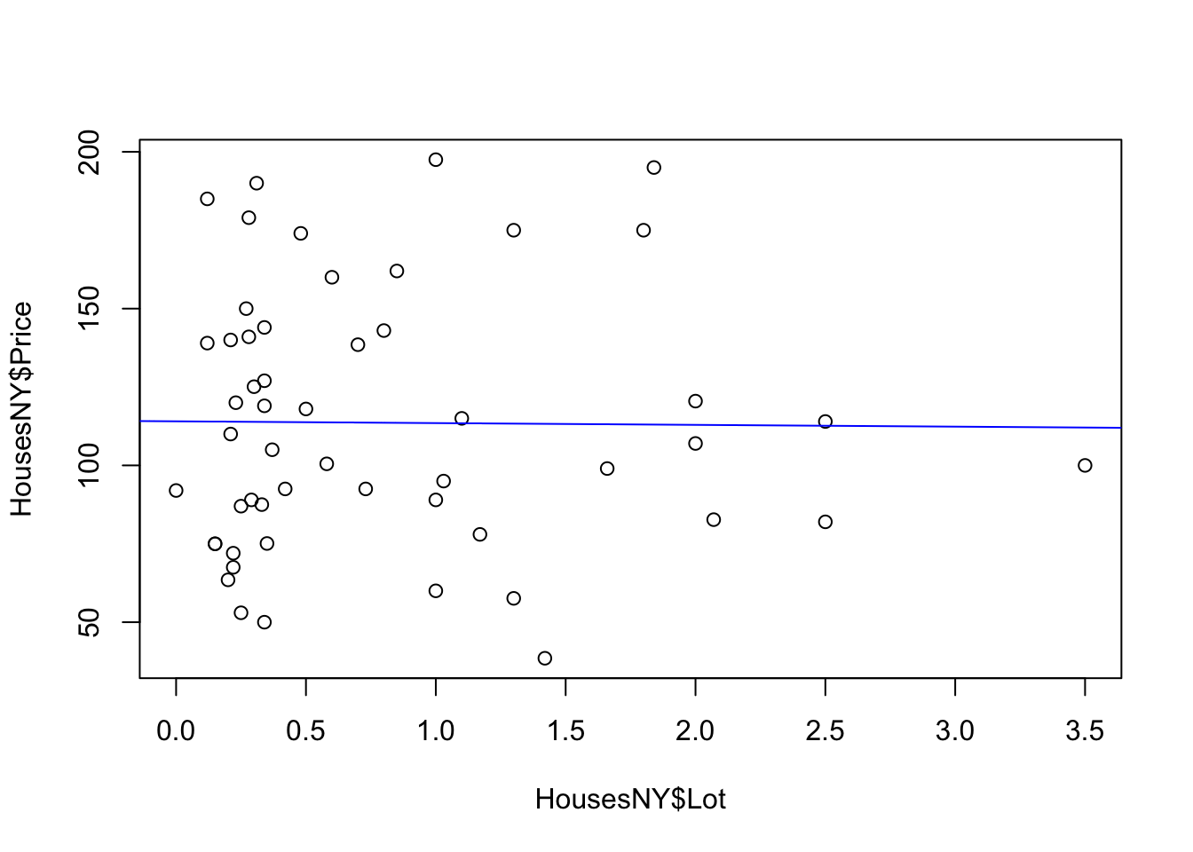 

For more professional plots, see the scatterplots tutorial

“Better” OLSRR regression output

If you want a different way of seeing the same output, you can use the ols_regress() command inside the olsrr package.

library(olsrr)

Attaching package: 'olsrr'

The following object is masked from 'package:equatiomatic':

    hsb

The following object is masked from 'package:datasets':

    rivers

Model1.lm.ols <- ols_regress(Model1.lm)
Model1.lm.ols

                          Model Summary                           
-----------------------------------------------------------------
R                        0.011       RMSE                 41.832 
R-Squared                0.000       Coef. Var            36.813 
Adj. R-Squared          -0.019       MSE                1749.910 
Pred R-Squared          -0.068       MAE                  34.152 
-----------------------------------------------------------------
 RMSE: Root Mean Square Error 
 MSE: Mean Square Error 
 MAE: Mean Absolute Error 

                               ANOVA                                 
--------------------------------------------------------------------
                 Sum of                                             
                Squares        DF    Mean Square      F        Sig. 
--------------------------------------------------------------------
Regression        9.983         1          9.983    0.006    0.9401 
Residual      89245.412        51       1749.910                    
Total         89255.395        52                                   
--------------------------------------------------------------------

                                    Parameter Estimates                                     
-------------------------------------------------------------------------------------------
      model       Beta    Std. Error    Std. Beta      t        Sig       lower      upper 
-------------------------------------------------------------------------------------------
(Intercept)    114.091         8.364                 13.641    0.000     97.300    130.882 
        Lot     -0.575         7.611       -0.011    -0.076    0.940    -15.855     14.705 
-------------------------------------------------------------------------------------------

The ols_regress command produces beautiful output, but sometimes it doesn’t work well with other commands. So I tend to run a lm command at the same time to have both available.

Sometimes, this command can produce a weird error:

This is probably because you loaded the moderndive package

This is probably because you loaded the moderndive package. They do not play nicely together. Save your work, restart R and do not run any line that says library(moderndive)!.