Lab 1: R intro
Welcome to Lab 1
The aim of this lab is to get comfortable in R and in R-Markdown, and to practice identifying some study jargon as we practiced in class. Lab instructions will be here and how-tos will be condensed into the Tutorial
The Canvas page for this lab is: https://psu.instructure.com/courses/2243429/assignments/14748231
If the labs are causing major problems with your computer or your computer hardware is struggling (or you have any other software issue), Talk to Dr Greatrex.
We can fix this and there are other options for “online R” that you can use.
Getting started
1a. Review the Lab Q&A
First, please review the lab Q&A: CLICK HERE. It explains
- What you need to submit
- How you are graded and where the rubric is
- The late policy
- What counts as cheating
1b. Follow Tutorial 1
Review CLICK HERE to see some of the powerful things we can do in R.
We will do this in class.
Your homework:
2. Make lab-Markdown
Create a new RMarkdown document called STAT462-Lab1-PSUID.Rmd. e.g. for me STAT462-Lab1-hlg5155.Rmd.
Delete any friendly welcome text so you have a blank space.
2a: Adding paragraphs & course late policy
You might find it easier to use the markdown visual text editor.
Click the “Visual” symbol at the top left of the document to switch.
In the white text area, create a level 1 Header called “Introduction to STAT-462”.
Leave a blank line, then use the STAT-462 syllabus to describe the course late policy in your own words (e.g. you’re writing about this in the white space).
Press “knit” at the top of the screen. If you haven’t made a mistake a pop up should appear with a html file and your edits. If you have a made a mistake, stop and fix before continuing or talk to a teacher.
3: Code showcase
<br<
Leave another blank line and add a new Level 1 Header called “Code Showcase”. Add a blank line afterwards too - the reason for all the blank lines is that R formatting often gets messed up with not enough blank lines, but it will ignore excess ones.
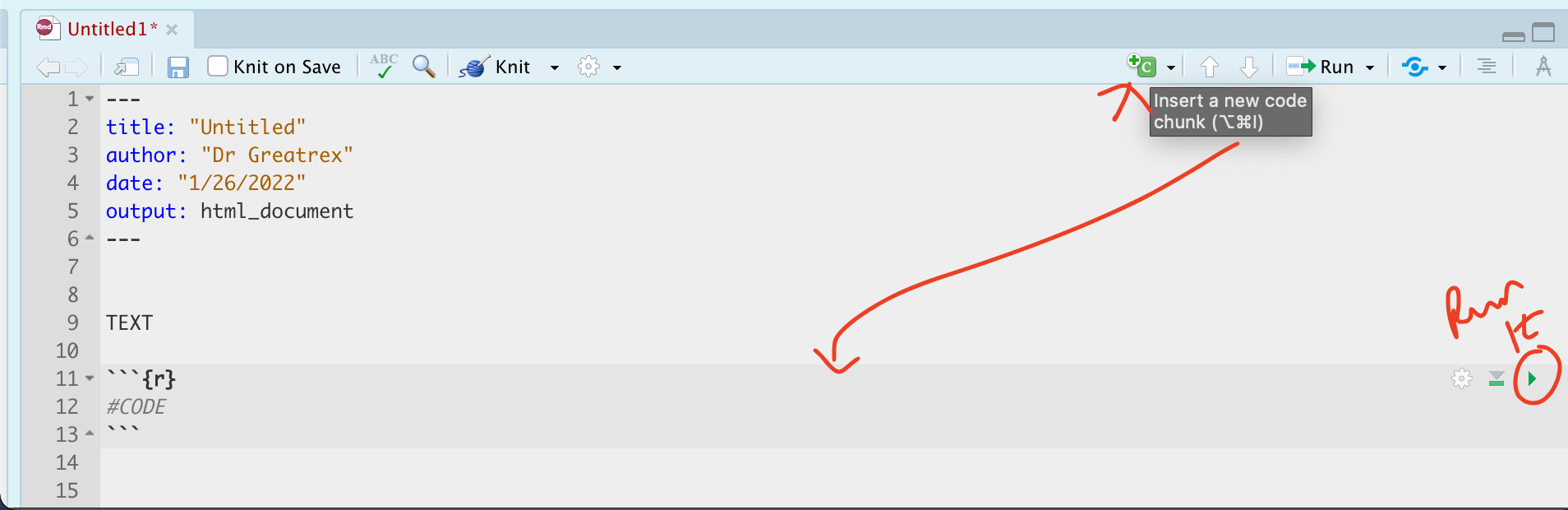
Create a code chunk. Inside use R code to calculate the following. You HAVE to show the code!
- 1033 (e.g
103*103*103, or103^3)
_ The co-sine of your age (google is your friend, google R function for cosine)
- Use R code to work out how many characters are in the longest town name in Wales Llanfairpwllgwyngyllgogerychwyrndrobwllllantysiliogogogoch.
- Hint 1, remember you can copy paste this into your code.
- Hint 2.. your tutorials and quote marks!
- Hint 3.. you can google any R command, try googling the “R command for number of characters in a word”.
- Hint 1, remember you can copy paste this into your code.
Press “knit” at the top of the screen. If you haven’t made a mistake a pop up should appear with a html file and your edits. If you have a made a mistake, stop and fix before continuing.
4. Packages
Today we will be using commands from several packages. Somewhere near the top of your script, make a new code chunk and add this code. We will probably have to install them first (see the tutorial)
Remember to run the code chunk! (pressing the green arrow, or go to the run button on the top right and press Run All)
library(tidyverse)
library(skimr)
library(ggplot2)
library(plotly)
library(ggpubr)
library(palmerpenguins)
5: Data analysis
5a Load & summarise the data
Leave a blank line, and create a new level 1 heading called Penguin Analysis. Leave a blank line afterwards too. We’re going to work with a table of data that’s already pre-loaded into R inside the ggplot2 package.
Make sure you have run the library code chunk above without error, or it won’t work.
Load the data using this command. You can ignore the raw penguin data
data("penguins")Type the
?penguinscommand in the console. This will bring up the help file.State the
- Object of Analysis
- A reasonable population you would be happy to apply this dataset to*
- Variables and units - you are allowed to copy these names/units from the help file
*Imagine you are giving this analysis to a newspaper editor. What population do you think this sample could represent?
5b Look at the data
Now look at the data itself. If you look in the environment tab, you will see a new variable called penguins Click on it’s NAME to see the spreadsheet/table itself and familiarise yourself with the data.
We could have also looked at the data by either by typing its name into the console, the command View(penguins) or a code chunk, or by using commands like head(penguins) to show the first few lines
5c. Summary analysis
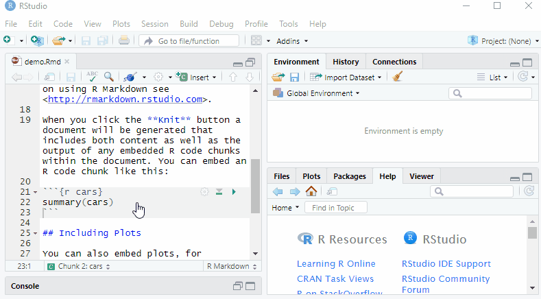
Let’s look at the summary statistics. Leave a blank line and create a new code chunk containing the following code
# mpg comes from the ggplot2 package
# skim comes from the skimr package
skim(penguins)
This command compiles the summary statistics for the penguin dataset - sometimes its easier to view this if you press the knit button and look at the html pop-up. You can also use the summary() command to achieve a similar result
summary(penguins)Summarise the dataset.
This should include:
- A short description of any missing data. For example, are there entire rows missing? Certain columns? Imagine you are using this dataset for modelling, are there rows that will need removing? etc etc? Try `View(penguins)` to look at the penguin dataset itself
- How many penguins were from 2008?
Hint, the table command..
Hint 2, to choose a column use the $ sign e.g. tablename$columnname
Hint 3, R IS CASE SENSITIVE!
- A histogram of one variable of your choice and a description of the variable.
E.g. unimodal? skewed? Any outliers? - A scatterplot between two variables of your choice and a description of the scatterplot
Hint https://allisonhorst.github.io/palmerpenguins/articles/examples.html *
*Hint 2, for a description, see this Khan page
- The correlation between two variables of your choice
- Hint, the cor command *
- Hint, the cor command *
- A correlation test fully written up in a way that a non expert would understand. For example you include the H0,the H1 the test statistic, the p value and your interpretation. I will let you choose your own significance threshold. You should also show the code output.
- *Hint, the cor.test command and see the Canvas correlation page for interpretations.
- *Hint, the cor.test command and see the Canvas correlation page for interpretations.
*In step 3 and 4 you are allowed to copy the code. There are two reasons for this. The first is that many of you are new to R, it’s lab 1 and I want you to get more exposure to what R looks like (and this is how I learn new coding techniques). The second is that we can spend weeks learning how to make a basic histogram, but now there are all of these amazing professional plots that can be made with a little more code, so I would prefer you spent your time learning them :)
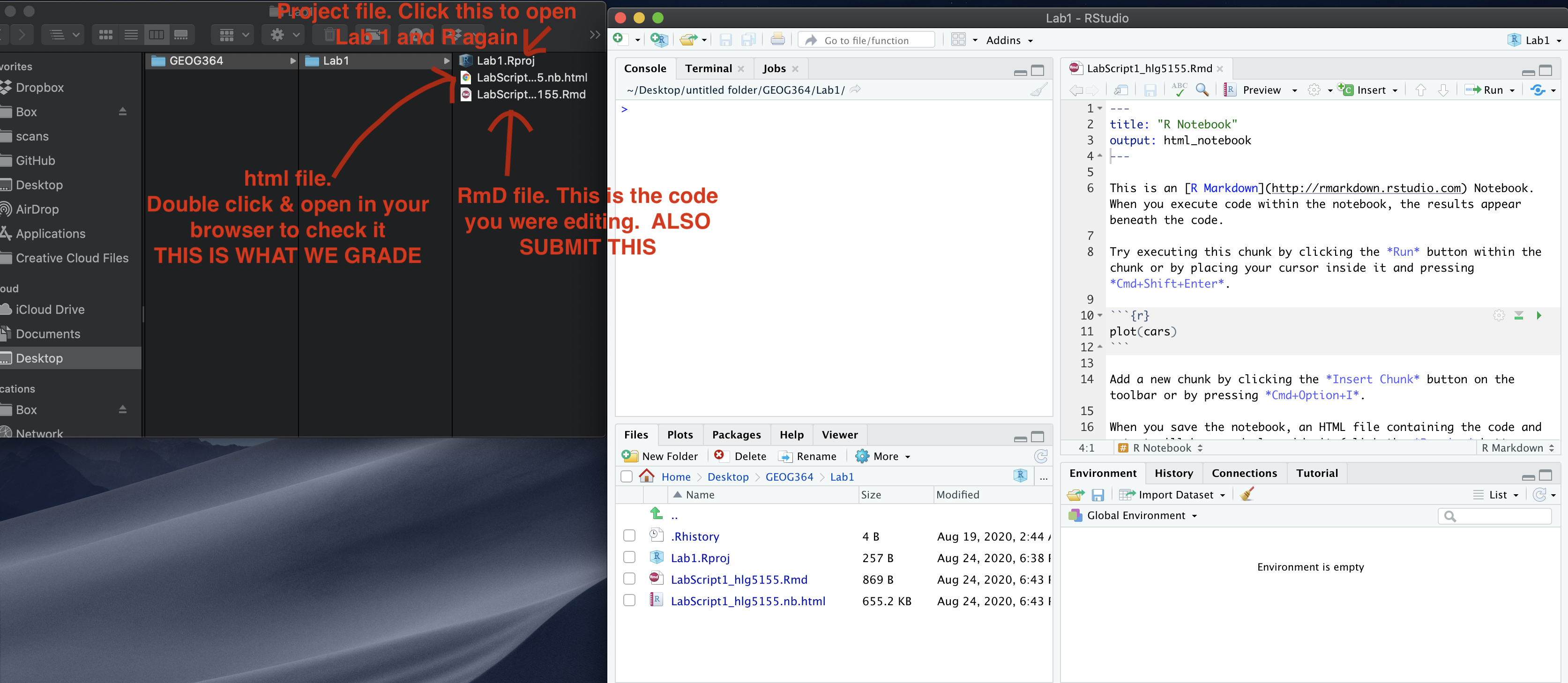
6. Submitting your Lab
Remember to save your work throughout and to spell check your writing (next to the save button). Now, press the knit button again. If you have not made any mistakes in the code then R should create a html file in your lab 1 folder which includes your answers. If you look at your lab 1 folder, you should see this there - complete with a very recent time-stamp.
In that folder, double click on the html file. This will open it in your web-browser.
CHECK THAT THIS IS WHAT YOU WANT TO SUBMIT.
If you are on R studio cloud, see Tutorial 1 for how to download your files
Now go to Canvas and submit BOTH your html and your .Rmd file in Lab 1.