# Load libraries
library("tidyverse") # Lots of data processing commands
library("knitr")     # Helps make good output files
library("ggplot2")   # Output plots
library("rmarkdown") # Helps make good output files
library("lattice")   # Makes nice plots
library("RColorBrewer") # Makes nice color-scales
library("skimr")     # Summary statistics
library("Stat2Data") # Regression specific commands
library("corrplot")  # correlation plots
library("GGally")    # correlation plots
library("ggpubr")    # QQplots
library("olsrr")     # Regression specific commands
library("plotly")    # Interactive plots
library("readxl")    # Read from excel files
library("equatiomatic") # extract equations
library("ggstatsplot") # Make nice plots
library("visreg") #visualise regression outputs
library("MASS") # Studentised residuals
## you may need additional libraries or to install some of these.
#Just install them and add them to this list if you get errors.Lab 5: MLR
Welcome to Lab 5
By the end of this week’s lab, you will be able to:
- Create Multiple Regression Models
- Assess Multiple Regression Models
- Model selection
The Canvas page for this lab is: https://psu.instructure.com/courses/2243429/assignments/14842792
If the labs are causing major problems with your computer or your computer hardware is struggling (or you have any other software issue), Talk to Dr Greatrex and REMEMBER YOU CAN ALWAYS USE RSTUDIO CLOUD.
Getting started - DO NOT SKIP
We will start removing style marks for lab write-ups that have missed this section
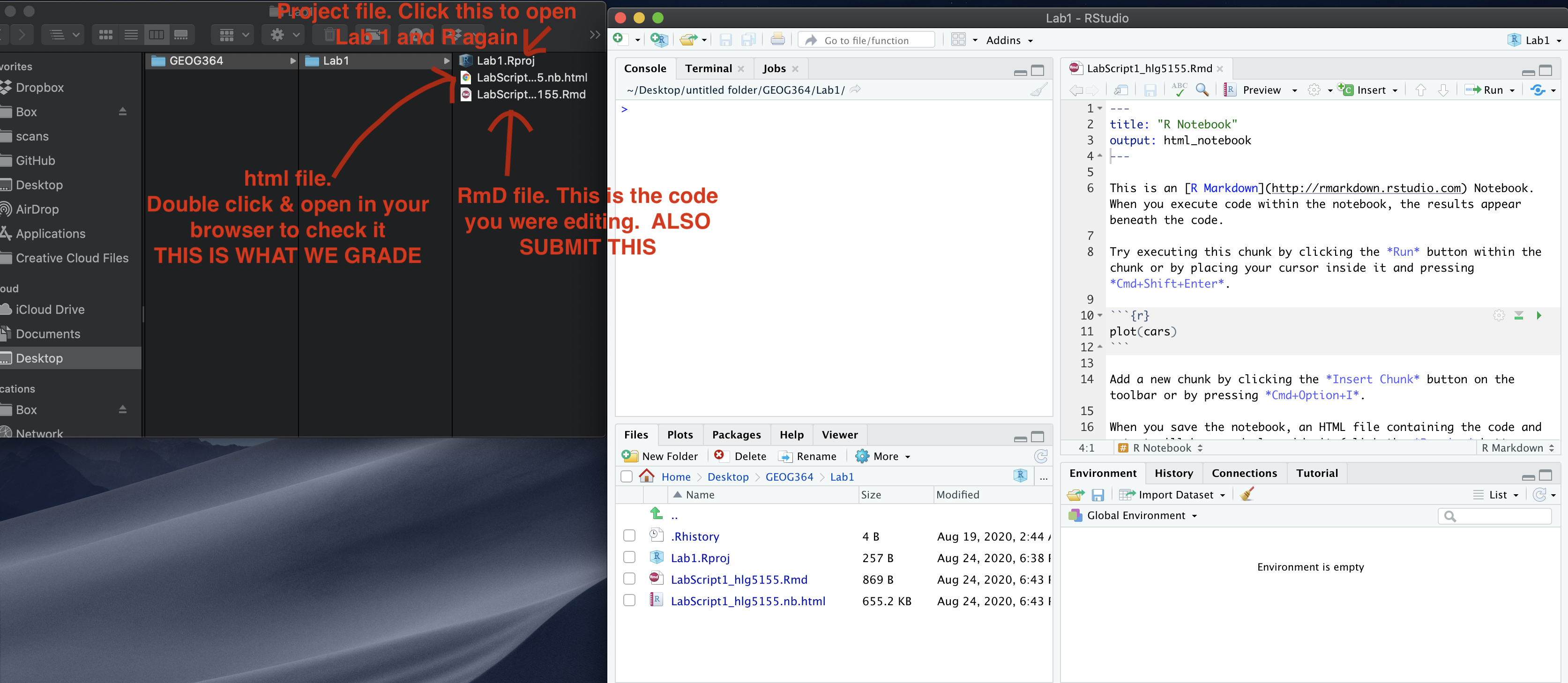
1. Make a new project and markdown file
Follow Tutorial 2 (link working) to create a new project and a new RMarkdown file that knits.
You should now have a new project and a new RMarkdown file that knits.
Create a code chunk near the top and load these packages. You may need to install them first using Tutorial 2.3 (Link working).
Step D: Finally, press knit to check the html works and your theme works.
IF YOU IGNORED STEP 1 ABOVE GO BACK AND DO IT! You lose marks for things like no theme, poor headings etc.
PART 2: Movie Ratings
2.1 Problem statement / Read in the data
You are an analyst for a Hollywood studio. The studio wants to understand how profitable a movie is.
You can access their training data file, Lab5_HollywoodMovies2011.csv from Canvas, which includes information on movies that came out of your Hollywood Studio in 2011.
| Variable Name | Description |
|---|---|
| RottenTomatoes | Percentage total rating from critical reviews on Rotten Tomatoes |
| AudienceScore | Percentage audience rating from opening weekend surveys |
| TheatersOpenWeek | Number of cinemas showing the movie on opening weekend |
| BOAverageOpenWeek | Average box office revenue per theater opening week-end, in dollars |
| DomesticGross | Gross revenue in the US by the end of 2011, in millions of dollars |
| Profitability | Percent of the budget recovered in profits. So 300 means 300% of the budget spent on making the movie was recovered as profit. |
Download the file from Canvas which contain the data. Use the read_csv command to read it into R and save it as a variable called movies.
2.2 Exploratory Analysis
In the text, identify the object/unit of observation, the response variable and re-create the table above to show the predictors. (Hint, you can click table on ‘visual mode’)
Use the corrplot command to fit a correlation matrix
ggcorrmat(movies)2.3 Fit the full MLR model
If you saved your data as a variable called movies, this code should let you fit a full ‘first-order’ multiple regression model to assess profitability. By full, I mean we’re including all predictors
# This is the same lm as before, and I'm just adding in Column names to the model
FullModel <- lm(Profitability ~ RottenTomatoes + AudienceScore +
                               TheatersOpenWeek + BOAverageOpenWeek +
                               DomesticGross, data = movies)

ols_regress(FullModel) # or summary(FullModel), whichever you prefer
Using the results above, write out the answers to these questions in FULL SENTENCES and your own words.
Identify how much data there is in the sample (n) and the number of predictors (k)
Either using equatiometric or alone, write out the full mathematical equation for this sample.
Use this code to look at LINE and outliers. In the text, summarise if you think the model meets the LINE assumptions and if there are any influential outliers. Don't worry about changing anything if it doesn't, just comment on your findings. Are you comfortable using this model for:
- Assessing the average profitability?
- Predicting the profitability of a new movie?
    # Check linearity and equal variance
    # plot the residuals
    ols_plot_resid_fit(FullModel)
    ols_plot_resid_stud(FullModel)
    ols_plot_resid_stand(FullModel)
    #Check normality
    ols_plot_resid_hist(FullModel)
    ols_test_normality(FullModel)
    ols_plot_resid_qq(FullModel)

    #Check for influential outliers
    ols_plot_resid_lev(FullModel)
Which predictor has the large effect on Profitability (not taking into account significance). Reflect on how that corresponds to your assessment from correlation matrix.
Using the model summary and a T-Test at a 10% level (otherwise called “partial slopes), identify which variables you would like to drop from the full model. Provide reasons for your choices. You do not have to write down hypothesis testing steps here.
2.4 Fit a reduced model
- Now, copy/paste your code from the full model and modify so that you only predict profitability given RottenTomatoes andDomesticGross. MAKE SURE TO SAVE YOUR LM TO A NEW MODEL NAME e.g. Model2.
# This is the same lm as before, and I'm just adding in Column names to the model
Model2 <- lm(Profitability ~ RottenTomatoes + DomesticGross, data = movies)

ols_regress(Model2) # or summary(Model2), whichever you prefer
Write down the mathematical equation for the estimated regression line.
Assess LINE and whether there are influential outliers. Don't worry about changing anything if it doesn't, just comment on your findings. Are you comfortable using this model for:
- Assessing the average profitability?
- Predicting the profitability of a new movie?
2.5 Compare the models
- What percentage of variability in profitability is explained by each model? Given just this statistic, which model would you choose? Why is the variability so low?
- Another way of comparing models is the Aikeke Information Criterion (AIC). Using https://online.stat.psu.edu/stat462/node/199/and the many great google tutorials out there, explain what AIC is and why it’s useful in comparing models. Using this method, which model would you choose?
AIC(FullModel,Model2)2.6 Finding the “optimal model”
There are many models/combinations of predictors that we could use to predict our response variable. We want to find the best model possible, but we also don't want to overfit.
So far, we manually compared two models. In fact there is a way to compare all the combinations of predictors. This is using the ols_step_best_subset() command.
Describe what the "best subset" method is doing. Hint, we will go over this in lectures, but also https://online.stat.psu.edu/stat501/lesson/10/10.3
Run this on your FULL linear model fit, FullModel. to assess the optimal fit.
BestSubsets <- ols_step_best_subset(FullModel)
BestSubsets
Using at least 3 goodness of fit measures, comment on which model is your final favourite.
Using the code from 2.3 and 2.4, fit your favourite model and take a quick look at LINE assumptions. As before, you don't need to find a new model if it's not valid (just talk about what you find)
Why are there suddenly variables in your "best" model that you likely dropped from your Full model at the end of 2.3.
PART 3 Bonus credit (beyond the lab)
This goes above and beyond Lab 7 - I will award up to 10 bonus points in general for completing the following task.
There are other ways of fitting a model than least squares. This includes the LASSO and RIDGE approaches which include regularization.
- Using the tutorials below, explain what each method is doing
- See if you can get either/both RIDGE or LASSO working in R to predict profitability. You might need to install new libraries
How do your models compare to your favourite least-squares model?
https://www.pluralsight.com/guides/linear-lasso-and-ridge-regression-with-r
https://www.r-bloggers.com/2021/05/lasso-regression-model-with-r-code/
This goes beyond our course, but I want to introduce those interested to it. Note, I reserve the right to award more than 10 points if it gets really complex!
PART 4 Submitting your Lab
Remember to save your work throughout and to spell check your writing (next to the save button).
Now, press the knit button for the final time.
If you have not made any mistakes in the code then R should create a html file in your lab 7 folder which includes your answers. If you look at your lab 7 folder, you should see this there - complete with a very recent time-stamp. In that folder, double click on the html file. This will open it in your browser. CHECK THAT THIS IS WHAT YOU WANT TO SUBMIT.
If you are on R studio cloud, see Tutorial 1 for how to download your files Now go to Canvas and submit BOTH your html and your .Rmd file in Lab 7.
PART 5. Grading Rubric/checklist
See the table below for what this means - 100% is hard to get!
HTML FILE SUBMISSION - 10 marks
RMD CODE SUBMISSION - 5 marks
Professional report 15 MARKS
Full marks for a report that I would take into a job interview. You have done things like fully labeled plots using words, tried more sophisticated plots than just the basics (remember ggstatplot!), written full paragraphs/sentences, used equation formats, sub-headings, used spell check, explained results in clear language, included units, used a theme and table of contents. You lose marks for each thing that makes it look non-professional.
Describe the data and EDA -8 MARKS
You have summarised the data and correctly created/interpreted the correlation matrix
Full model - 8 MARKS
You created the model correctly. In your write up you have summarised the model equation (including the coefficients as numbers) & summarising units afterwards. You have produced a model summary, assessed LINE/outliers and answered all questions as appropriate.
Model Fit - 8 MARKS
You have assessed which variables do not add to the model using partial slopes/T-tests.
New model, making the model - 8 MARKS
You have correctly refitted and interpreted the model, answering all questions as appropriate.
Stepwise - 8 MARKS
You have found the “optimal model” and commented on what the best subset command is doing. You have compared the models using 3 goodness of fit metrics
Above and beyond - This will be added to extra credit (see part 4)
See above
[70 marks total]
Overall, here is what your lab should correspond to:
| Grade | % Mark | Rubric |
|---|---|---|
| A* | 98-100 | Exceptional. Not only was it near perfect, but the graders learned something. THIS IS HARD TO GET. |
| NA | 96+ | You went above and beyond |
| A | 94+: | Everything asked for with high quality. Class example |
| A- | 90+ | The odd minor mistake, All code done but not written up in full sentences etc. A little less care |
| B+ | 87+ | More minor mistakes. Things like missing units, getting the odd question wrong, no workings shown |
| B | 84+ | Solid work but the odd larger mistake or missing answer. Completely misinterpreted something, that type of thing |
| B- | 80+ | Starting to miss entire/questions sections, or multiple larger mistakes. Still a solid attempt. |
| C+ | 77+ | You made a good effort and did some things well, but there were a lot of problems. (e.g. you wrote up the text well, but messed up the code) |
| C | 70+ | It’s clear you tried and learned something. Just attending labs will get you this much as we can help you get to this stage |
| D | 60+ | You attempt the lab and submit something. Not clear you put in much effort or you had real issues |
| F | 0+ | Didn’t submit, or incredibly limited attempt. |