Tutorial 6: Input/Output
GEOG-364 - Spatial Analysis
Tutorial 6: Input/Output
This tutorial is all about reading in and saving files
Tutorial 6A: Reading in Excel Files
R can easily read in Microsoft Excel spreadsheets using the readxl package:
Basic approach
- Make sure the readxl package is loaded.
E.g. islibrary(readxl)in your library code chunk?
Have you run the code chunk?
- Place your excel file in your project folder.
E.g. for Lab 2, place frostdays.xlsx into your Lab 2 project folder.
Make a new code chunk and add the read_excel() command e.g.
frost <- read_excel("frostdays.xlsx")Here the command is
read_excel(), you are applying this to “frostdays.xlsx” (e.g. reading in that file), then assigning the result to a variable called frost. Because you are using your project, R knows to look inside your project folder to find the file.
If this works, there should be no errors and nothing prints on the screen when you run the code chunk.
In the environment tab, frost should have appeared with a description as a table with 76 rows (observations/obs), and 7 columns (variables). In R, this type of table/spreadsheet is called a data.frame.
Example
For example, for our frostdata.xlsx data in Lab 2:
# Read in the frost.xlsx file in your projexct folder and assign it to a variable called frost
frost <- read_excel("frostdata.xlsx")
# Check the column names, or click on its name in the Environment quadrant
names(frost)## [1] "Station" "State" "Type_Fake"
## [4] "Avg_DOY_SpringFrost" "Latitude" "Longitude"
## [7] "Elevation" "Dist_to_Coast"# frost is a standard table, to make a spatial version and save it to a variable called frost.sf
frost.sf <- st_as_sf(frost, coords=c("Longitude","Latitude"),crs=4326)
# and plot the SF spatial version
tmap_mode("view")
qtm(frost.sf,dots.col="Elevation")Troubleshooting
It says it can’t find the file: - Are you running the right project? e.g. does it say Lab 2 at the top of the screen? - Did you put the file into your Lab 2 folder? - Did you spell it right and include the full .xslx extension? - Did you use quote marks?
It says read_excel doesn’t exist - Did you install the readxl package? - Did you load the readxl package? Go click the code chunk with the library command again! - Did you spell the command right? (case sensitive) - Did you use () afterwards so R understands that it’s a command?
Using the wizard.
Sometimes you just can’t get it working. In those cases, try the import wizard.
- Go to the file menu at the very top of the screen. Click import dataset, then From Excel. Use the wizard to find your file and get it looking correct. It will show you the code you need in the code preview
- Because we want to include this file in the markdown, rather than pressing OK, copy the code preview text and put it in your code chunk.
Tutorial 6B: Reading in csv Files
These are comma separated text files, you can read them into microsoft excel.
Basic approach
- You don’t need any special package to read in a csv file
- Make sure there is the
library(sf)andlibrary(tmap)in your library code chunk at the top of the script to plot
- Place the csv file into your project folder
- Use the
read_csv()command to read it into R.
- Make sure to assign it to a variable or it will just print onto the screen
- Run the code chunk, then click on the variable name in the Environment quadrant to check that it read in correctly (especially make sure that column names have read in correctly)
Worked example
For example, for to read in a csv file on PA fossils, convert it to spatial and make a map:
# Read in the frost.xlsx file in your projexct folder and assign it to a variable called frost
fossil <- read.csv("PA_fossils.csv")
# Check the column names, or click on its name in the Environment quadrant
names(fossil)## [1] "Key" "Name" "Period" "Long" "Lat"# brazil is a standard table, to make a spatial version and save it to a variable called frost.sf
# I get the coords from the column names
fossil.sf <- st_as_sf(fossil, coords=c("Long","Lat"),crs=4326)
# and plot the SF spatial version
tmap_mode("view")
qtm(fossil.sf,dots.col="Period")Tutorial 6C: Reading in “Shape Files”
These are even easier to enter into R, BUT it is important to understand what a shapefile actually is first. They are designed to hold vector spatial data (points, polygons, lines.. etc), so the projection and coordinates are already loaded.
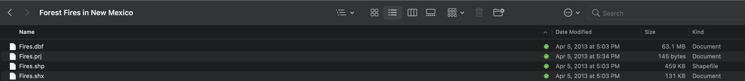
A “shapefile” is in fact a COLLECTION of files, often zipped together. Each sub-file has a different extension, for example, TOGETHER, all these files equals a “shapefile”. Sometimes there might be only 3 or 4 subfiles, sometimes several more, but they will all have the same file name. For example, here is a shapefile of forest fires in New Mexico.
Basic approach
Shapefiles can be points, lines or polygons - the same method works for all of them. To read it in:
- Put ALL the sub-files in your project folder OR IT WILL NOT WORK
- Make sure there is the
library(sf)andlibrary(tmap)in your library code chunk at the top of the script to plot
- Use the
st_read()command to load the .shp file directly into an sf format
- To see the data table, simply click on its name
Worked example
To read in that forest fire data.
# ONLY WORKS IF ALL THE SUBFILES ARE THERE.
# Reading directly into sf format
fires.sf <- st_read("fires.shp")## Reading layer `Fires' from data source
## `/Users/hlg5155/Dropbox/My Mac (E2-GEO-WKML011)/Documents/GitHub/Teaching/Geog364-2021/Fires.shp'
## using driver `ESRI Shapefile'
## Simple feature collection with 16383 features and 32 fields
## Geometry type: POINT
## Dimension: XY
## Bounding box: xmin: -109.0456 ymin: 31.3323 xmax: -103.0722 ymax: 36.9986
## Geodetic CRS: WGS 84# But you can still treat it like a standard table
# Here i print the first 6 rows
head(fires.sf)## Simple feature collection with 6 features and 32 fields
## Geometry type: POINT
## Dimension: XY
## Bounding box: xmin: -106.562 ymin: 33.1551 xmax: -104.4505 ymax: 35.1978
## Geodetic CRS: WGS 84
## ID ORGANIZATI UNIT SUBUNIT SUBUNIT2 FIREID FIRENAME FIRENUMBER FIRECODE
## 1 1 BIA SWR NMMEA 0 345134 A&BSECTION 1302 <NA>
## 2 2 BIA SWR NMMEA 0 345135 SALTWELL 1303 <NA>
## 3 3 BLM NM NMROD 0 90146 RED BLUFF <NA> 4751
## 4 4 BIA SWR NMMEA 0 345136 PETERSON 1304 <NA>
## 5 5 BIA SWR NMMEA 0 345137 TREASTANK 1305 <NA>
## 6 6 BIA SWR NMSPA 0 333494 JACK 1601 <NA>
## CAUSE SPECCAUSE STATCAUSE SIZECLASS SIZECLASSN PROTECTION FIREPROTTY FIRETYPE
## 1 Human 0 0 A 1 1 11 1
## 2 Human 0 0 A 1 1 11 1
## 3 Human 0 0 B 2 1 11 1
## 4 Human 0 0 A 1 1 11 1
## 5 Human 0 0 A 1 1 11 1
## 6 Human 0 0 A 1 1 11 1
## YEAR_ STARTDATED CONTRDATED OUTDATED GACC DISPATCH GACCN STATE
## 1 1980 1980-03-07 1980-03-07 1980-03-07 SWCC Lincoln Zone 110 New Mexico
## 2 1980 1980-03-17 1980-03-17 1980-03-17 SWCC Lincoln Zone 110 New Mexico
## 3 1980 1980-03-19 1980-03-19 1980-03-19 SWCC Lincoln Zone 110 New Mexico
## 4 1980 1980-03-22 1980-03-22 1980-03-22 SWCC Lincoln Zone 110 New Mexico
## 5 1980 1980-03-23 1980-03-23 1980-03-23 SWCC Lincoln Zone 110 New Mexico
## 6 1980 1980-03-25 1980-03-25 1980-03-26 SWCC Albuquerque Zone 110 New Mexico
## STATE_FIPS FIPS DLATITUDE DLONGITUDE TOTALACRES TRPGENCAUS TRPSPECCAU
## 1 35 35 33.1551 -105.8005 0.1 8 27
## 2 35 35 33.2534 -105.7005 0.1 3 10
## 3 35 35 33.5834 -104.4505 3.0 9 30
## 4 35 35 33.1551 -105.7839 0.1 4 11
## 5 35 35 33.1862 -105.7155 0.1 8 27
## 6 35 35 35.1978 -106.5620 0.1 4 12
## geometry
## 1 POINT (-105.8005 33.1551)
## 2 POINT (-105.7005 33.2534)
## 3 POINT (-104.4505 33.5834)
## 4 POINT (-105.7839 33.1551)
## 5 POINT (-105.7155 33.1862)
## 6 POINT (-106.562 35.1978)# and plot the SF spatial version
tmap_mode("view")
qtm(fires.sf,dots.col="DISPATCH")Shapefiles can be points, lines or polygons - the same method works for all of them. For example, to read in the borders:
# ONLY WORKS IF ALL THE SUBFILES ARE THERE.
# Reading directly into sf format, you can see it's a POLYGON file
NM_border.sf <- st_read("New_Mexico.shp")## Reading layer `New_Mexico' from data source
## `/Users/hlg5155/Dropbox/My Mac (E2-GEO-WKML011)/Documents/GitHub/Teaching/Geog364-2021/New_Mexico.shp'
## using driver `ESRI Shapefile'
## Simple feature collection with 1 feature and 53 fields
## Geometry type: POLYGON
## Dimension: XY
## Bounding box: xmin: -109.0496 ymin: 31.3324 xmax: -103.0015 ymax: 37.00027
## Geodetic CRS: WGS 84# and plot the SF spatial version
tmap_mode("view")
# turn off the interactive and plot
tmap_mode("plot")
qtm(NM_border.sf, fill= grey(0.9)) +
qtm(fires.sf,dots.col="DISPATCH") +
tm_legend(legend.outside=TRUE)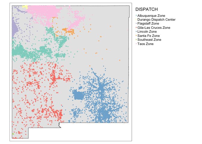
Tutorial 6D: Reading in raster/field data: geoTifs
Field data is stored differently because there needs to be a value for every single location. It is typically storeds as a geoTif (.tif) or a netCDF (.nc). Luckily, the raster package can easily cope with both:
Basic approach
- Put your geotif into your project folder
- NEW: Make sure there is the
library(raster)in your library code chunk at the top of the script to plot
- Use the
raster()command to load the .tif file directly into an sf format. Sometimes you will get a warning like the one shown below. Ignore it
- and plot. There are many ways to plot raster data in R. Here are a few: https://datacarpentry.org/r-raster-vector-geospatial/02-raster-plot/
Worked example
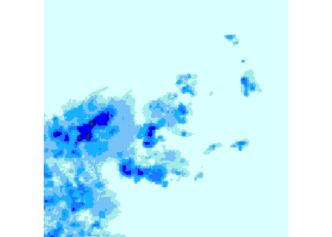
To read in a geotif for the rainfall over Africa on May-2-2001:
# the file is in my project folder
rain_210502.raster <- raster("RFE_Africa_20210521.tif")To plot:
plot(rain_210502.raster)
Tutorial 6E: Reading in US Census Data
This section was updated with the kind permission of Dr Noli Brazil. We can use R to directly open any census/American community survey data at any scale for any geography. It’s pretty cool.
6E.a Finding data online: Policy Map
Before we start, let’s take a quick look at what is available online. The site we’ll use in this lab is called PolicyMap. Penn State provides access to this for all students.
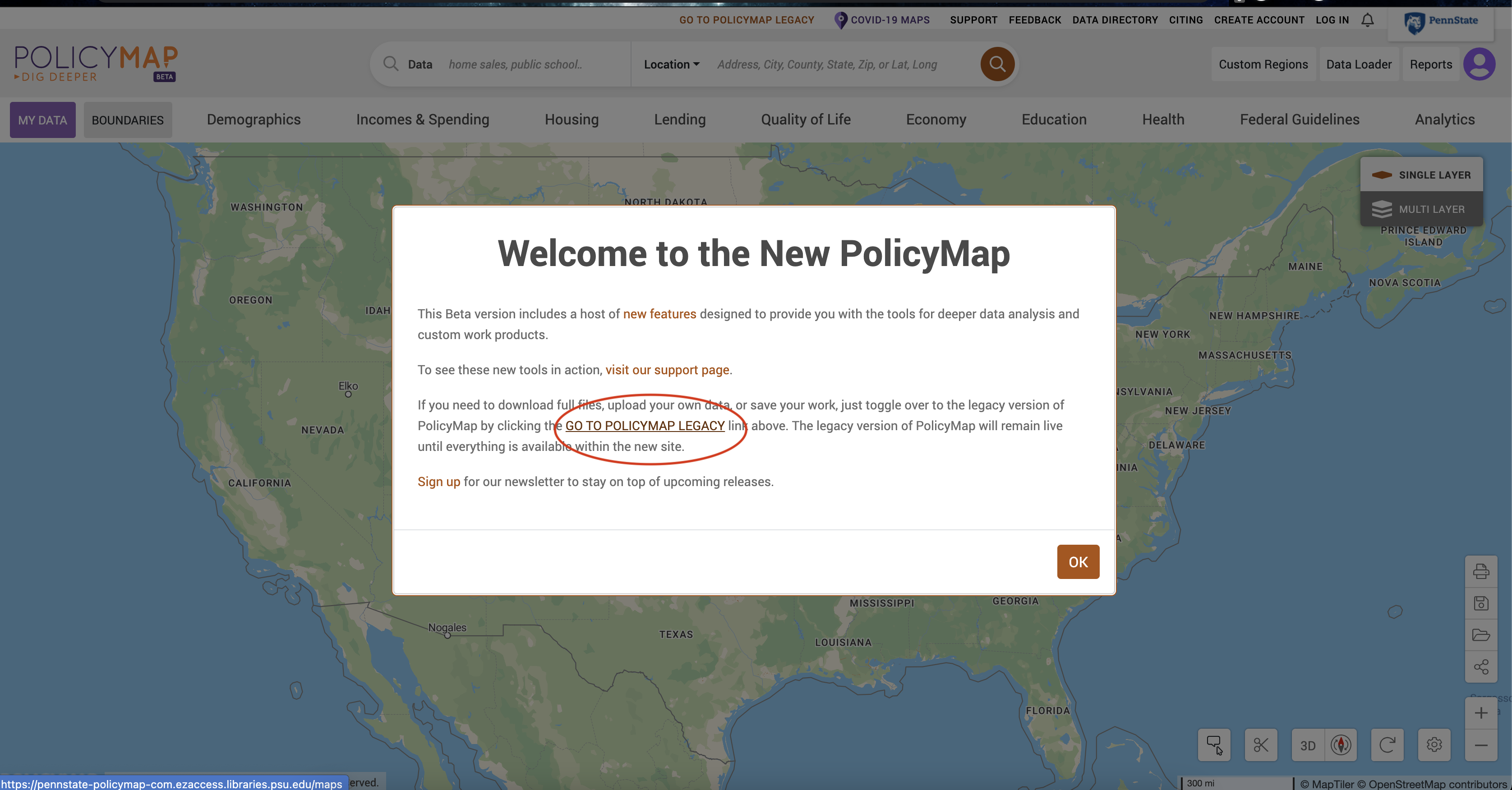
To access it, go here: https://libraries.psu.edu/databases/psu01762 (or search for Penn State Library policy map) and click access policy map. Log in
You should see something like the picture below, note if you want to download data you currently need to click the Legacy button, we are just browsing so click OK
You should see a Location search bar somewhere near the top of the page. Type in “Pennsylvania” in the search bar and Pennsylvania (State) should pop up as the first selection. Click it.
Now have a look around and see what features are available to map. For example, go to the educational achievement tab and choose attainment then percentage with at least a bachelors degree. You should get something like this.
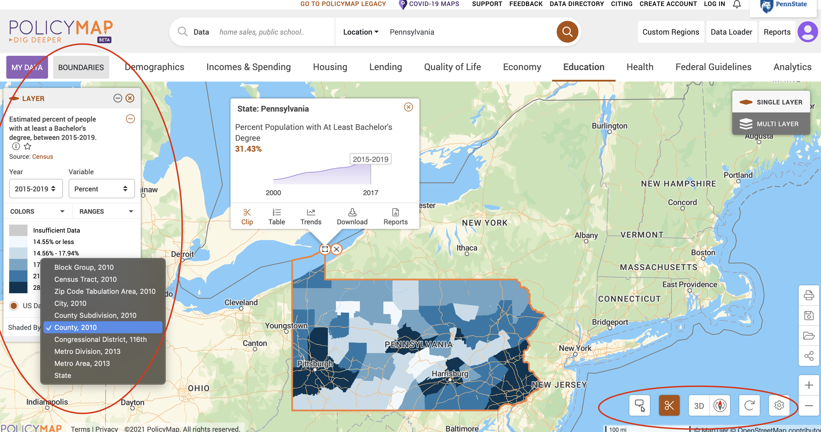
I also cropped to the PA boundaries, bottom right
Here you can change many things, like the unit of observation and when the data was collected. It’s a really powerful programme and if you simply need a quick pretty plot, there is nothing faster.
It’s also possible to download csv files containing the data (To see how, see the instructions here: https://crd150.github.io/lab3.html). However, we are now going to read the census data directly into R.
6E.b Loading Census data in R
To load census data in R, you need a password from the US census website - and then to load it into R each time.
Sign up (you should have already done this)
You can easily access US census data within R, but you need to sign up in advance for a password.
https://api.census.gov/data/key_signup.html
You can use Penn State as the organisation. This is just you promising that you will follow the terms and conditions when using this data. In a few minutes, e-mail you a personal access code called an API key. Click the link in the e-mail to activate.
Sometimes your key will just stop working - it’s fine to simply sign up for a new one
Teach R your API key
You don’t need to type this password in every time you run R. Instead we will teach it to R once.
- Save everything and run
library(tidycensus)
- IN THE CONSOLE, type this command, but replace “YOUR API KEY GOES HERE” with the password you were given
#census_api_key("YOUR API KEY GOES HERE", install=TRUE,overwrite=TRUE)
# Here is an imaginary example, you need your own number
# census_api_key("d2a990f429205c51b54998ec58886c6cf01a7ef2", install=TRUE,overwrite=TRUE)- This wll now load the password. If you run this command several times or it is in your script, it will give an error. This is a one off process.
- CLOSE R-STUDIO AND RE-OPEN YOUR PROJECT FILE
Find what variables are there
First, make sure that library(tidycensus) and library(VIM) are in your library code chunk and you have run it.
We are going to focus on installing demographic data from the American Community Survey using the tidycensus package. The American Community Survey is a huge dataset for the US Population at Census tract scale. There are variables from population density, to demographic data, to employment and economic indicators.
We don’t want to download all the data, so to see what variables are available to us, we will use the following command. This will take some time to run.
#tidycensus package
Variables_2017 <- load_variables(2017, "acs5", cache = TRUE)Now click on the name Variables_2017 in the Environment tab to take a look.
To search for specific data, select “Filter” located at the top left of this window and use the search boxes that pop up. For example, to match our web-search, look inside concept for bachelors and you should see all people with a bachelors degree is code “B15012_001”.
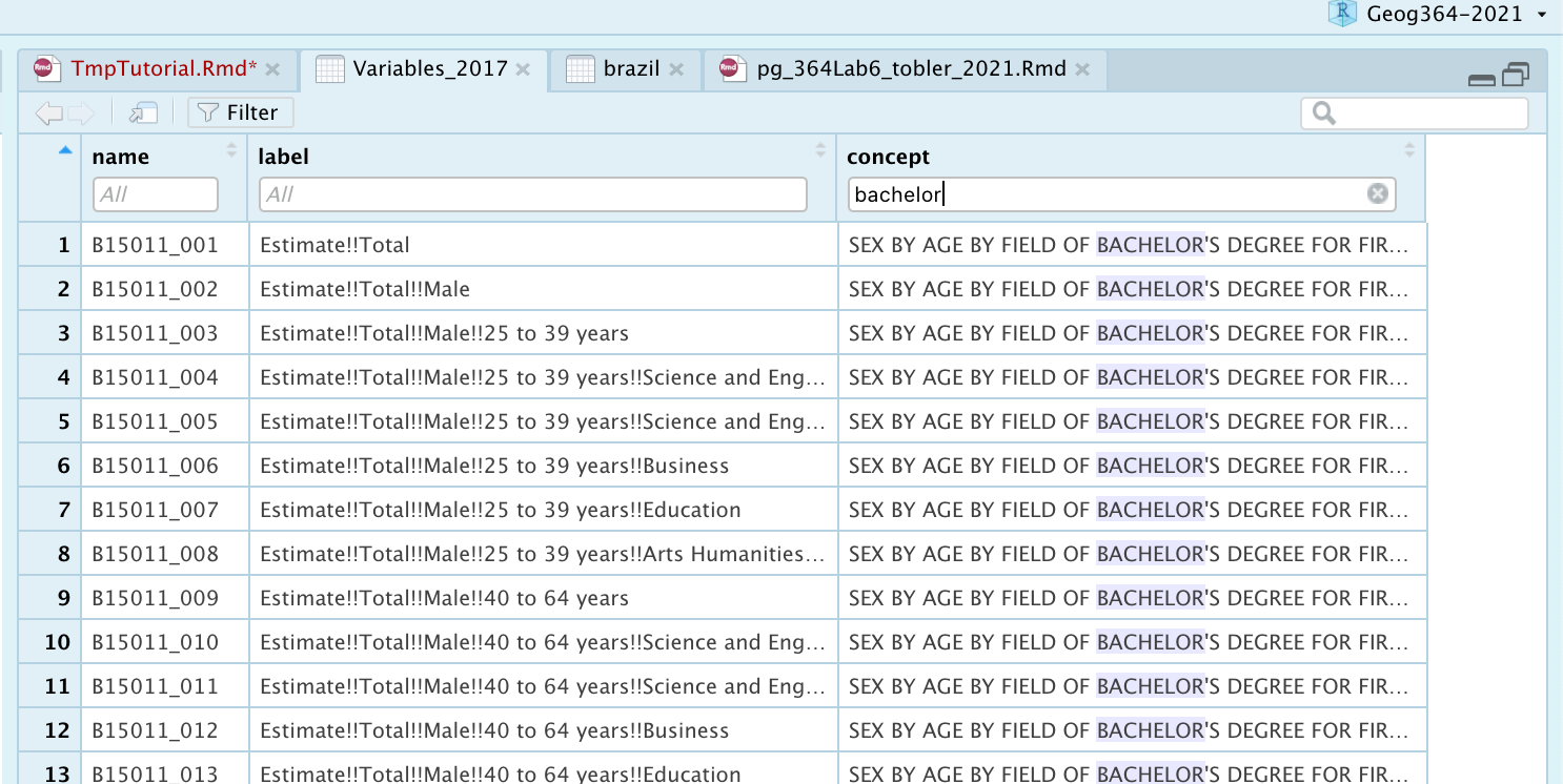
Alternatively, I found the codes on this website: https://www.socialexplorer.com/data/ACS2017_5yr/metadata/?ds=ACS17_5yr. Frustratingly I don’t think they store the codes on policy map. You can see some more common codes in my example below
6E.c The get_acs command
Now we have the ID for those commands, we want to download the data itself.
- The command/function for downloading American Community Survey (ACS) Census data is
get_acs(). - The command for downloading decennial Census data is
get_decennial().
They have similar arguments
Some important notes - READ THESE FOR LAB 7
This command can take a minute to start running
I strongly suggest results=FALSE in the code chunk option at the top to stop all the “processing” text in your final report (AKA in the place you put message=FALSE, warning=FALSE or add a figure caption)
SEE HERE FOR A FULL TUTORIAL: https://walker-data.com/tidycensus/articles/basic-usage.html - this tells you how to edit the parameters.
If you add new variables, make sure they are inside the parentheses for the variable argument! A common error is to add them as a new line, not adding to the list of variables.
In the code below, we specified the following arguments.
- geography: The level of geography we want the data in; in our case, the county. Other geographic options can be found here: https://walker-data.com/tidycensus/articles/basic-usage.html
- year: The end year of the data (because we want 2013-2017, we use 2017).
- variables: The variables we want to bring in as specified in a vector you create using the function c(). Note that we created variable names of our own (e.g. “topop”) and we put the ACS IDs in quotes (“B03002_003”). Had we not done this, the variable names will come in as they are named in the ACS, which are not very descriptive.
- state: We can filter the counties to those in a specific state. Here it is c(“PA”, “NY”) for Pennsylvania and New York. If we don’t specify this, we get all counties in the United States - this is a HUGE download. When we cover Census tracts in the next lab, a county filter will also be available.
- survey: The specific Census survey were extracting data from. We want data from the 5-year American Community Survey, so we specify “acs5”. The ACS comes in 1-, 3-, and 5-year varieties.
- geometry: If geometry is set to FALSE, it just brings in a standard table. If it’s set to true, it makes it an sf file.
- wide: This makes on column for each variable, setting it to false would make one single column for all the estimates and one for the margin of error. We normally want wide=TRUE
- geography: The level of geography we want the data in; in our case, the county. Other geographic options can be found here: https://walker-data.com/tidycensus/articles/basic-usage.html
Here is an example:
# Download PA ACS data at county level for some chosen variables, using tidycensus
# see the helpfile for get_acs for more options
PA_NY.ACS.sf <- get_acs(geography = "county",
year = 2017,
variables = c(total.population = "B05012_001", # total population
total.house = "B25001_001", # total housing units
house.value = "B25075_001", # house value
identity.native = "B02001_004", # total who identify as native american
identity.hisp = "B03003_003", # total who identify as Hispanic
identity.CentralA= "B03001_008", # total who identify as Hispanic Central A
identity.SouthA = "B03001_016", # total who identify as Hispanic South A
identity.white = "B03002_003", # total who identify as white
identity.black = "B03002_004", # total who identify as black
med.income = "B19013_001", # median income
income.gt75 = "B06010_011", # number of people making > 75000 USD
for.born = "B05012_003", # number of foreign born people
house.age = "B25035_001", # average house age
month.house.cost = "B25105_001", # monthly house expenditures
med.gross.rent = "B25064_001", # median rent
total.workhome = "B08101_049", # number who work from home
owneroccupied = "B25003_002", # total owner occupied
total.beds = "B25041_001", # total number of beds in the house
broadband = "B28002_004", # total with broadband access
lackingplumbing = "B25047_003", # total without plumbing
completeplumbing = "B25047_002", # all mobile homes -
mobilehomesall = "B25024_010", # native mobile homes
mobilehomenative = "B25032E_010",# total with complete plumbing
total.bachdegree = "B15012_001" ) , # total with at least a bachelors degree
# SEE I ENDED THE VARIABLE LIST PARENTHESES
# AND USE THE COMMA TO MOVE ONTO THE OTHER VARS
state = c("PA","NY"),
survey = "acs5",
geometry = TRUE,
output="wide")
6E.d Understanding the ACS command output
Estimate vs margin of error
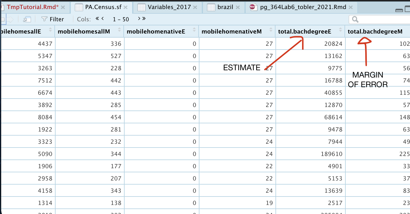
If you click on the name PA_NY.ACS.sf, you should now see that it has downloaded each one of your variables for every county in New York and PA. In fact, for every one, it has downloaded the ESTIMATE, but also has included the MARGIN-OF-ERROR, the 90% confidence interval on our result (90% of the time our result should be within this margin of error)
Calculate rates and densities
Finally, we currently have the TOTAL number of people/houses/beds/things in each county, but it is also useful to have the percentage. To calculate these we simply use the mutate command. If mutate doesn’t make sense, see this tutorial: https://crd150.github.io/lab2.html#Creating_new_variables
# Use the mutate functions, divide each total by the population and make a new column
PA_NY.ACS.sf <- mutate(PA_NY.ACS.sf, percent.income.gt75E = income.gt75E / total.populationE)
PA_NY.ACS.sf <- mutate(PA_NY.ACS.sf, percent.for.bornE = for.bornE / total.populationE)
PA_NY.ACS.sf <- mutate(PA_NY.ACS.sf, percent.nativeE = identity.nativeE / total.populationE)
PA_NY.ACS.sf <- mutate(PA_NY.ACS.sf, percent.hispE = identity.hispE / total.populationE)
PA_NY.ACS.sf <- mutate(PA_NY.ACS.sf, percent.CentralAE = identity.CentralAE/ total.populationE)
PA_NY.ACS.sf <- mutate(PA_NY.ACS.sf, percent.SouthAE = identity.SouthAE / total.populationE)
PA_NY.ACS.sf <- mutate(PA_NY.ACS.sf, percent.whiteE = identity.whiteE / total.populationE)
PA_NY.ACS.sf <- mutate(PA_NY.ACS.sf, percent.blackE = identity.blackE / total.populationE)
PA_NY.ACS.sf <- mutate(PA_NY.ACS.sf, percent.workhomeE = total.workhomeE / total.populationE)
PA_NY.ACS.sf <- mutate(PA_NY.ACS.sf, percent.bachdegreeE = total.bachdegreeE / total.populationE)
# or the mutate functions, divide each total by the number of houses and make a new column
PA_NY.ACS.sf <- mutate(PA_NY.ACS.sf, percent.owneroccupiedE = owneroccupiedE / total.houseE)
PA_NY.ACS.sf <- mutate(PA_NY.ACS.sf, percent.broadbandE = broadbandE / total.houseE)
PA_NY.ACS.sf <- mutate(PA_NY.ACS.sf, percent.mobilehomesallE = mobilehomesallE / total.houseE)
PA_NY.ACS.sf <- mutate(PA_NY.ACS.sf, percent.lackingplumbingE = lackingplumbingE / total.houseE)We can also work out the population density per unit area
First we need the spatial area of each census tract. We can do this using the st_area() command, then use mutate again to add the population density column
#Finding the area of each county
area.m2 <- st_area(PA_NY.ACS.sf)
# This is in metres^2. Convert to Km sq
area.km2 <- set_units(area.m2, "km^2")
area.km2 <- as.numeric(area.km2)Calculate the population density and the housing density per county:
PA_NY.ACS.sf <- mutate(PA_NY.ACS.sf, pop.densityE = total.populationE/area.km2)
# and the housing density
PA_NY.ACS.sf <- mutate(PA_NY.ACS.sf, house.densityE = total.houseE/area.km2)Change projections
Let’s check the map projections.
raster::projection(PA_NY.ACS.sf)## [1] "+proj=longlat +datum=NAD83 +no_defs"OK it appears to be in long/lat. As this is simply an sf file, we can do things like change the map projection, or any of the filters/joins you have learned in previous labs.
Often for census data it is good to use Tutorial 11 to transform your data to the UTM projection, which is what I have done here:
# NEED A BETTER PROJECTION
PA_NY.ACS.sf <- st_transform(PA_NY.ACS.sf,26916)Now with everything you learned about tmap (https://mgimond.github.io/Spatial/mapping-data-in-r.html#tmap), you will allow you to make some cool plots.
Here’s simply one example:
# create map 1
map1 <- tm_shape(PA_NY.ACS.sf, unit = "mi") +
tm_polygons(col="total.populationE",
style="pretty", legend.hist = TRUE,
palette="Reds") +
tm_layout(main.title = "Population per county in NY and PA", main.title.size = 0.75, frame = FALSE) +
tm_layout(legend.outside = TRUE)
map2 <- tm_shape(PA_NY.ACS.sf, unit = "mi") +
tm_polygons(col="pop.densityE",
style="pretty", legend.hist = TRUE,
palette="YlGnBu") +
tm_layout(main.title = "Population density per county in NY and PA (ppl per km2)", main.title.size = 0.75, frame = FALSE) +
tm_layout(legend.outside = TRUE)
tmap_options(check.and.fix = TRUE)
tmap_arrange(map1,map2)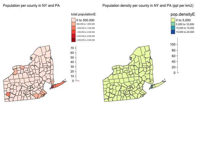
# create map 1
map3 <- tm_shape(PA_NY.ACS.sf, unit = "mi") +
tm_polygons(col="percent.bachdegreeE",
style="pretty", legend.hist = TRUE,
palette="Blues") +
tm_layout(main.title = "Percentage with a bachelors degress", main.title.size = 0.95, frame = FALSE) +
tm_layout(legend.outside = TRUE)
map4 <- tm_shape(PA_NY.ACS.sf, unit = "mi") +
tm_polygons(col="percent.lackingplumbingE",
style="pretty", legend.hist = TRUE,
palette="YlGnBu") +
tm_layout(main.title = "Percentage of houses without plumbing", main.title.size = 0.95, frame = FALSE) +
tm_layout(legend.outside = TRUE)
tmap_options(check.and.fix = TRUE)
tmap_arrange(map3,map4)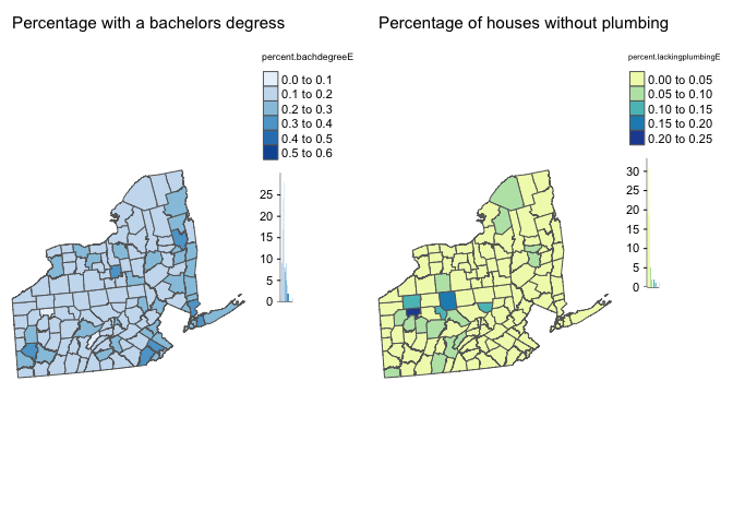
There are a load more ideas here: http://zevross.com/blog/2018/10/02/creating-beautiful-demographic-maps-in-r-with-the-tidycensus-and-tmap-packages/
Website created and maintained by Helen Greatrex. Website template by Noli Brazil