Lab 4: Manipulating Spatial Data

Welcome to Lab 4!

The aim of this lab is start getting more comfortable making high quality maps and manipulating data. We will also learn about some new markdown techniques for “inline code” and adding equations By the end of the lab you will be able to.

1. Use inline code commands
1. Insert an equation into your text and data
1. Make beautiful spatial plots
1. Read in shapefiles and manipulate your data spatially
1. Re-analyse your new york data

Assignment 4 is due by midnight the night before your next lab on Canvas. Your job is to submit the requirements on this page.

See your canvas assignment here. E.g go to canvas for assignment guidelines.

Need help? Add a screenshot/question to the discussion board here: LAB 4 DISCUSSION BOARD

A: Set up the lab

Set up R-Studio in the same way as before, creating a project file and a blank markdown document.
This will be the last time I am going to spell it out.

Step 1
Open R-Studio.
Create a new R-Project in your GEOG-364 folder called GEOG364_Lab4_PROJECT.
Reminder: Tutorial 2C: Projects.

Step 2
Go on Canvas to the Lab 4 page and download any datasets as needed (ozone.csv)
Put it/them in your GEOG364_Lab4_PROJECT folder. See the lab 3 instructions for how it should look.

Step 3
Make a copy of the lab template:
1. If you’re on your own computer:
  - Make a COPY of the template Rmd file.
  - Rename the COPY GEOG364_Lab4_userID_CODE.Rmd e.g. for me GEOG364_Lab3_hlg5155_CODE.Rmd
  - Move GEOG364_Lab4_userID_CODE.Rmd into your GEOG364_Lab4_PROJECT folder.
1. If you’re using R-studio cloud.
  - MAKE SURE YOU WENT TO YOUR WORKSPACE AND MADE A LAB 4 PROJECT!
  - Click on your Lab 4 project folder
  - In the files tab, click the check box by your template file, click More/Export & download it.
  - Click on Workspaces (top left) and enter your Lab 4 project folder.
  - In the files tab, click upload and upload the template
  - Now click the check box by the template file and rename to GEOG364_Lab4_userID_CODE.Rmd
    e.g. for me GEOG364_Lab4_hlg5155_CODE.Rmd

In both cases, your “Lab 4” R-Studio should look like this but for lab 4. If not ASK FOR HELP

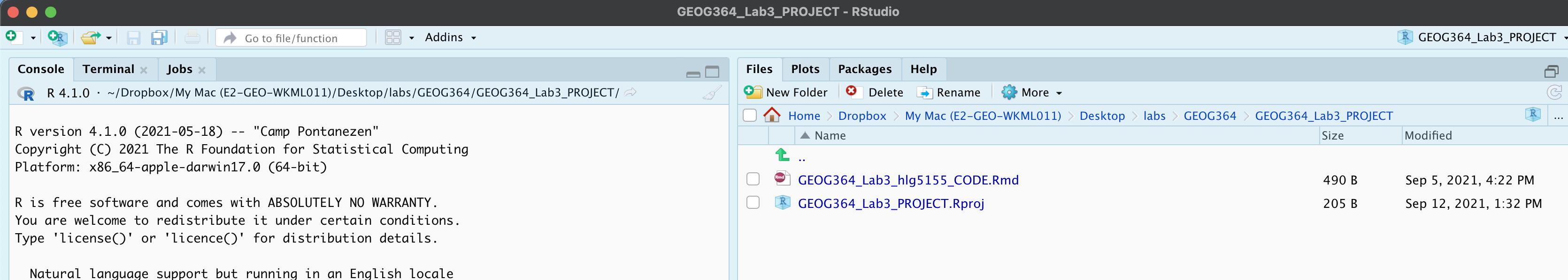
This is for lab 3 but you get the idea.

IMPORTANT! Did you open R via your lab 4 project file? If R-studio isn’t “looking in” your lab 4 folder in Files, or doesn’t have your lab 4 project name on the logo/at the top of the screen, close R studio, go to your lab 4 folder and double click the .Rproj to open your lab 4 project

Step 4
Click on your lab 4 .Rmd file in the files tab to open the script
(You should not have to search if you are in your Lab 4 project):
- Change the title to Lab 4.
- Change the theme if you like
- Edit the library code chunk so it looks like this:
```
library(knitr) 
library(tidyverse)
library(sf)
library(sp)
library(tmap)
library(skimr)
library(rnaturalearth)
library(readxl)
```
- Add in message=FALSE and warning=FALSE inside the top code chunk (see screenshot below) to remove the packages printing all the text
- If you accidentally messed up something remember you can re-copy your YAML code or options from a previous lab.
  The easiest way to do this is to navigate on your computer to that lab folder then double click the project file for the old lab to open an entirely new version of R-Studio for that lab. Then nothing gets confused
  equally on the cloud, make a new tab in your browser, go to your workspace (top left), and open the other project there
- Press knit.

You screen should now look like this but for Lab 4 and your options. If so,congrats
If not, ASK FOR HELP.

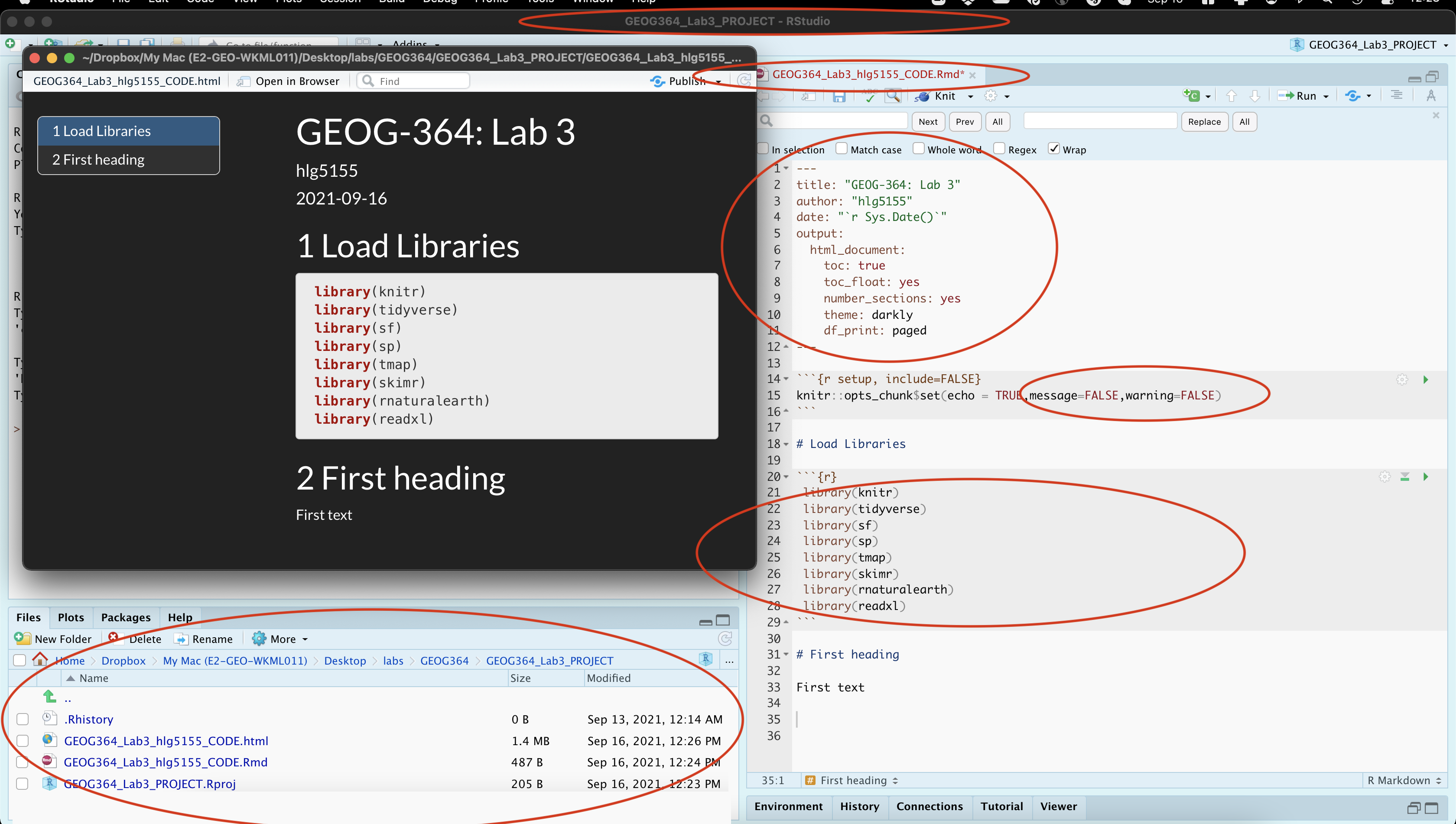
Note, your message=FALSE and warning = FALSE can go in the general options like my screenshot, or in the code chunk options for the library chunk

B: Markdown Edits

We are now going to insert “inline code” along with mathematical equations:

Step 5: Visual editor
Read the section: Tutorial 4G: Visual Editor to turn on the markdown visual editor (near the top of 4G)

Step 6: Inline code
Follow the new inline-code tutorial in Tutorial 4F: Inline Code to understand about inline code

Step 7: Equations
Follow Tutorial 4I: Equations to understand about adding equations.

Step 8:
Make a new section called Markdown.
Feel free to use subsections, numbers, font formats throughout to make it look professional as possible
IF YOU SKIPPED STEPS 6,7,8, GO DO THEM.

Step 9:
Now, attempt the following tasks, which are building on those tutorials but also on what you learnt in Labs 1,2 & 3:
TUTORIAL 4: MARKDOWN HAS THE ANSWERS.
1. Visual editor
  Write a short paragraph to explain the difference between pattern and process (See Lecture 5A & Sullivan chapter pdf).
  Use the visual editor to play with the fonts & formats.
  [you are being graded on the paragraph content not the format, so go wild]
2. Inline code
  - COPY your frost data from Lab 2 to your Lab 4 folder.
  - In a code chunk, read in the data to a variable called frost.
  - In the same code chunk, calculate
    - the mean of the Elevation column
    - the number of rows
    - the number of columns( hint nrow() and ncol())
    - Save the answers to sensibly named variables e.g. frost.elev,frost.nrow….
  - Edit the code chunk options so that the code and output are invisible when you press knit (you will still see them in the editing window).
  - In the text make a new paragraph, that says
    “In lab 2, we read in a dataset called frostdata.xlsx. The data has XXXX rows and YYYY columns, The mean of the Elevation column is ZZZZ UNITS.”.
    
    Replace XXXX, YYYY and ZZZZ with inline code that creates the answers automatically and UNITS with the appropriate units.
3. Rounding
  Your mean elevation is to too many decimal places in your sentence.
  Use the round() command to round your output to a sensible number of significant figures.
  To do this:
  - See this tutorials below on round (or google) https://www.datasciencemadesimple.com/round-function-in-r/
  - Make a new copy of your sentence about frost,
  - Now edit the inline code chunk to round the mean of the elevation to an appropriate number of decimal places for your units.
  - Your final sentence should look something link this but about your frost data and with a good number of decimal places for your units.
    
    “In the inbuilt starwars dataset, there are 87 rows and 14 columns. The average height of a character is 174.4 cm.”
4. Equations
  In a new paragraph, describe the Z score and include the equation properly formatted.

C: Better spatial plots

This is the final “lego” lab e.g. where it is more about building blocks than statistics. So let’s improve our maps. There are some wonderful tutorials online, much better than I could write. So we shall work through one of them

Step 10:
Tutorial script.
We need a place for you to work through the tutorial. Follow step 3 to make a new copy of your lab template and put it in the Lab 4 folder.This time, call your copy GEOG364_MapTutorial.Rmd

You do NOT have to submit your tutorial file

Step 11:
Work through the tutorial.
Go here: https://mgimond.github.io/Spatial/mapping-data-in-r.html
Work through the mapping tutorial at that page, copying the code into code chunks in your tutorial lab script, checking it works and trying to understand why each line of code is there.
Step 12:
Once you are done, close your tutorial script so that you don’t accidentally edit it for your Lab 4.

D: Ozone & MAUP

Lab Background

As cities increase in size, it is important to understand atmospheric air pollution. Two major pollutants include Ozone (O3) and particulates (PM 2.5). In this lab, we will map them and explore their impact on populations in California.

Ozone is a naturally occurring molecule made up of three Oxygen atoms. 90% of the plant’s ozone exists in the “ozone layer”, which exists approximately 20-25km above sea level, in the stratosphere. Stratospheric ozone is crucial for human life, as it absorbs damaging solar ultra-violet radiation (see the “ozone hole” for the importance of natural ozone).

However, 10% of the planet’s ozone is found in the lowest levels of the atmosphere, in the air which we breathe. It is created when pollutants such as NOx and VOCs (emitted by cars and industry) react with sunlight.

Strong evidence exists that the risk of premature death increases with increased amounts of low-level-ozone.Too much ozone can cause immediate health problems such as asthma. Over the longer term, ozone exposure can exacerbate pre-existing lung and heart health problems. It is therefore important to map the spread of ozone to support public health policy.

To explore this issue, ozone measurements were taken across the State of California. Population density has also been recorded at each site using this source: https://sedac.ciesin.columbia.edu/data/set/gpw-v4-population-density-rev11.

*The units of the ozone measurements are in “1000 parts per billion”.
*The units of population density are people per square km.

Basics

Step 13:
Read the ozone.csv data into R and assign to a variable called ozone.
hint! Like HW4 you need a the read.csv() command instead of the read_excel one. Tutorial here if you’re stuck (https://www.datacamp.com/community/tutorials/r-data-import-tutorial)

Step 14: Summary Statistics…
This is week 4, you know the drill! Explore the data and tell me professionally in the text:

Tell me more about Ozone pollution and health. What’s the big deal (feel free to use REFERENCED pictures/screenshots)
Tell me what you know about the data/study. Imagine you are a journalist or a policy maker - be critical! If some aspect of the “meta data” (the data source, author, population etc.) is missing, make sure to note it.
Tell me about the data you just read into R e.g.
- What is the unit of observation for this data
- Is the data marked? If so, what are the marks? (e.g. what columns are there)
- How many observations are there? (e.g. how many rows)
- What are the summary statistics - do they look reasonable?
- What does the histograms of the ozone column look like (remember to get the exact column name you can use the command names(ozonedata))?
- Use a QQ-Norm to plot to assess if the data in the ozone column is normally distributed. (hint, see the QQQplot here http://www.sthda.com/english/wiki/normality-test-in-r if you want a prettier one)
- BONUS! Conduct and interpret in full sentences, a Wilks-Shapiro test to assess if the data is normal (hint: tutorial: http://www.sthda.com/english/wiki/normality-test-in-r)

Step 15: Research hypothesis…
From what you (now) know about ozone, how do you expect the pattern of ozone to be distributed over California? What influences it and what are confounding factors?

Spatial mapping

Step 16: Convert to spatial…
Make a new code chunk
Use Reminder: Tutorial 11Bb convert-to-sf: Projects to do the following:

Look at the ozone data and note the colunm names containing the x and y coordinates (CASE SENSITIVE)
Convert ozone to sf format and assign the result to a variable called ozone.sf
hint, the current map projection is Lat/Long 4326
Check it works. use the command plot(st_geometry(ozone.sf)) to make sure it converted OK. Hint, to understand what I was asking last week with st_geometry, also try plot(ozone.sf) and plot(ozone$LONGITUDE,ozone$LATITUDE)

Step 17: First map…
Use the previous labs and tutorials to make an interactive map of ozone levels. Use the layers button to explore the data. Does the distribution agree with what you expected? (hint, rural Joshua Tree has some of the highest Ozone levels..)

Step 18: Download county borders
Make a new code chunk
Use this code to download county borders for California and plot to check (ignore the warnings). Luckily for us they are in the same map projection. you should see something like this:

ca_counties.sf <- us_counties(states="CA")
  
plot(st_geometry(ca_counties.sf))
plot(st_geometry(ozone.sf),add=TRUE,col="red",pch=16,cex=.5)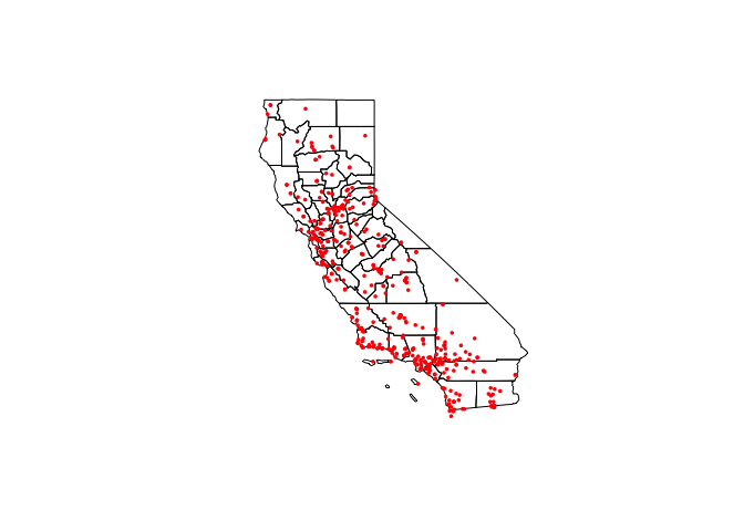

Step 19: Download congressional borders
Make a new code chunk
Use this code to download congressional borders for California and plot to check (ignore the warnings). Luckily for us they are in the same map projection. you should see something like this:

ca_congress.sf <- us_congressional(states="CA")

plot(st_geometry(ca_congress.sf))
plot(st_geometry(ozone.sf),add=TRUE,col="red",pch=16,cex=.5)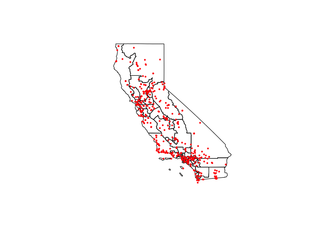

Here are my prettier tmaps of population density over ozone tracts.

# Plot the population density data, the col is the column name
# You can run the command tmaptools::palette_explorer() in the console and choose a more appropriate palette (you will need to install the shinyjs package)
tmap_mode("view")
tm_shape(ca_congress.sf) + tm_borders() +
  tm_shape(ozone.sf) +
  tm_dots(col="POPULATION_DENSITY", palette = "YlOrRd", 
          title="Population density (people/km^2)", size=0.04) +
  tm_legend(legend.outside=TRUE)+
  tm_basemap(leaflet::providers$OpenStreetMap.DE)

# Plot the population density data, the col is the column name
# No basemaps are possible in static mode, which is frustrating
tmap_mode("plot")
tm_shape(ca_congress.sf) + tm_borders() +
  tm_shape(ozone.sf) +
  tm_dots(col="POPULATION_DENSITY", palette = "YlOrRd", 
          title="Population density (people/km^2)", size=0.04) +
  tm_legend(legend.outside=TRUE)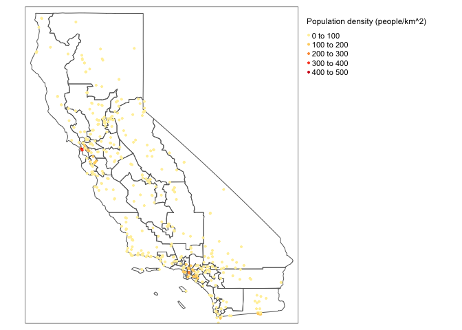

Step 20: Make prettier maps
Given my code here and your tutorials, make some better maps of the ozone levels at your California sites, overlayed with the COUNTY borders.
(hint the column name is OZONE_1000PPB..)

Spatial wrangling

Finally, let’s assess how to summarise our data across polygons using the st_join command

Putting this into a tutorial broke the website, so let’s add it here.

Step 22:Get it running on your computer
Copy the code below into a code chunk in your lab script. Run each line and see if you can understand what is going on. Check it knits and that you can see the same maps in your lab output.

First many people have had issues with the USBoundaries packages. Let’s reinstall: a. Save your work and close R studio. Open a fresh r studio window. b. copy and run these commands in the console. They should work

install.packages("USAboundaries")
install.packages("rgeos")
install.packages("remotes")
remotes::install_github("ropensci/USAboundariesData")
remotes::install_github("ropenscilabs/rnaturalearthhires")

 c. Close and reopen your Lab 4 project (go to the lab 4 folder and double click your .RProj file). In R, go to the files tab, reopen your .Rmd code and press run all. It should now work.

OK let’s continue

# First, look at the ozone column names to understand that table
head(ozone.sf)

## Simple feature collection with 6 features and 5 fields
## Geometry type: POINT
## Dimension:     XY
## Bounding box:  xmin: -124.163 ymin: 34.4622 xmax: -119.7402 ymax: 40.8019
## Geodetic CRS:  WGS 84
##   LOCATION                   SITE_NAME   SHORT_NAME OZONE_1000PPB
## 1     2001 Citrus Heights-Sunrise Blvd Citrus_Hghts      24.93750
## 2     2008            El Capitan Beach El_Capitan_B      31.37524
## 3     2011          Eureka-Fort Avenue Eureka-FtAve      17.20210
## 4     2012         Fresno-Cal State #2 Fresno-ClSt2      36.64366
## 5     2013      Fresno-Drummond Street Fresno-Drmnd      28.07397
## 6     2016     Carmel Valley-Ford Road Carm_Val-Frd      26.86707
##   POPULATION_DENSITY                  geometry
## 1         39.6102759 POINT (-121.2711 38.6988)
## 2          0.1215512 POINT (-120.0258 34.4622)
## 3         17.5800110  POINT (-124.163 40.8019)
## 4         54.4619531 POINT (-119.7402 36.8136)
## 5         81.1287549 POINT (-119.7413 36.7055)
## 6          2.2620163 POINT (-121.7333 36.4819)

#----------------------------------------------------------
# Now look at the ca_congress.sf column names, 
# You can see there are a load of random columns
# From googling, I worked out that the congressional 
#   district column is cd116fp
#-----------------------------------------------------------
head(ca_congress.sf)

## Simple feature collection with 6 features and 12 fields
## Geometry type: MULTIPOLYGON
## Dimension:     XY
## Bounding box:  xmin: -122.5181 ymin: 32.57796 xmax: -116.9281 ymax: 37.81649
## Geodetic CRS:  WGS 84
##    statefp cd116fp      affgeoid geoid                  namelsad lsad cdsessn
## 11      06      14 5001600US0614  0614 Congressional District 14   C2     116
## 15      06      44 5001600US0644  0644 Congressional District 44   C2     116
## 24      06      38 5001600US0638  0638 Congressional District 38   C2     116
## 27      06      46 5001600US0646  0646 Congressional District 46   C2     116
## 28      06      15 5001600US0615  0615 Congressional District 15   C2     116
## 29      06      53 5001600US0653  0653 Congressional District 53   C2     116
##         aland    awater state_name state_abbr jurisdiction_type
## 11  673063887 827178439 California         CA             state
## 15  207102703  65976773 California         CA             state
## 24  262677141   3804835 California         CA             state
## 27  187028152    995827 California         CA             state
## 28 1549309488  73721922 California         CA             state
## 29  352382739   5270106 California         CA             state
##                          geometry
## 11 MULTIPOLYGON (((-122.5181 3...
## 15 MULTIPOLYGON (((-118.3333 3...
## 24 MULTIPOLYGON (((-118.1513 3...
## 27 MULTIPOLYGON (((-117.9979 3...
## 28 MULTIPOLYGON (((-122.1403 3...
## 29 MULTIPOLYGON (((-117.1887 3...

#-----------------------------------------------------------
# We are first going to stick these together to make a table where I know the 
# zone every point is in. 
#-----------------------------------------------------------
joineddata  <- st_join(ozone.sf, ca_congress.sf)

#-----------------------------------------------------------
# Now I'm going to do a load of statistics on the joined data
# We are forcing R to use the commands from the dplyr package
#-----------------------------------------------------------

# How many observations in each congressional district
number.obs    <-  joineddata %>%  
                   dplyr::group_by(cd116fp) %>% 
                   dplyr::summarize(number.obs = length(cd116fp)) %>% 
                   dplyr::select(number.obs)

# Mean population density in each congressional district
mean_POPULATION_DENSITY <-   joineddata %>%  
                             dplyr::group_by(cd116fp) %>% 
                             dplyr::summarize(mean_POPULATION_DENSITY = mean(POPULATION_DENSITY)) %>% 
                             dplyr::select(mean_POPULATION_DENSITY)
                   
# Max population density in each congressional district
max_POPULATION_DENSITY <-    joineddata %>%  
                             dplyr::group_by(cd116fp) %>% 
                             dplyr::summarize(max_POPULATION_DENSITY = max(POPULATION_DENSITY)) %>% 
                             dplyr::select(max_POPULATION_DENSITY)

# Max population density in each congressional district
mean_OZONE_1000PPB    <-   joineddata %>%  
                           dplyr::group_by(cd116fp) %>% 
                           dplyr::summarize(mean_OZONE_1000PPB = mean(OZONE_1000PPB)) %>% 
                           dplyr::select(mean_OZONE_1000PPB)

#-----------------------------------------------------------
# And finally, merge them with the congressional polygon variable
# I'm first making a copy so that I don't mess anything up
#-----------------------------------------------------------
ca_congress.data.sf <- ca_congress.sf

ca_congress.data.sf <- st_join(ca_congress.data.sf, number.obs)
ca_congress.data.sf <- st_join(ca_congress.data.sf, mean_POPULATION_DENSITY)
ca_congress.data.sf <- st_join(ca_congress.data.sf, max_POPULATION_DENSITY)
ca_congress.data.sf <- st_join(ca_congress.data.sf, mean_OZONE_1000PPB)

#-----------------------------------------------------------
# And test plot, note I'm now plotting ca_congress.data.sf!
#-----------------------------------------------------------
plot1 <- qtm(ca_congress.data.sf,fill ="mean_POPULATION_DENSITY")
plot2 <- qtm(ca_congress.data.sf,fill ="max_POPULATION_DENSITY")
tmap_arrange(plot1,plot2)

plot3 <- qtm(ca_congress.data.sf,fill ="number.obs")
plot4 <- qtm(ca_congress.data.sf,fill ="mean_OZONE_1000PPB")
tmap_arrange(plot3,plot4)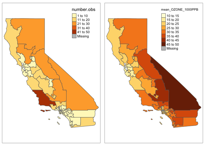

#-----------------------------------------------------------
# And finally take a look at the column names of the new sf variable - you can see
# our calculations have been added in
#-----------------------------------------------------------
head(ca_congress.data.sf)

## Simple feature collection with 6 features and 16 fields
## Geometry type: MULTIPOLYGON
## Dimension:     XY
## Bounding box:  xmin: -122.5181 ymin: 32.57796 xmax: -116.9281 ymax: 37.81649
## Geodetic CRS:  WGS 84
##    statefp cd116fp      affgeoid geoid                  namelsad lsad cdsessn
## 11      06      14 5001600US0614  0614 Congressional District 14   C2     116
## 15      06      44 5001600US0644  0644 Congressional District 44   C2     116
## 24      06      38 5001600US0638  0638 Congressional District 38   C2     116
## 27      06      46 5001600US0646  0646 Congressional District 46   C2     116
## 28      06      15 5001600US0615  0615 Congressional District 15   C2     116
## 29      06      53 5001600US0653  0653 Congressional District 53   C2     116
##         aland    awater state_name state_abbr jurisdiction_type number.obs
## 11  673063887 827178439 California         CA             state          1
## 15  207102703  65976773 California         CA             state          3
## 24  262677141   3804835 California         CA             state          3
## 27  187028152    995827 California         CA             state          6
## 28 1549309488  73721922 California         CA             state          4
## 29  352382739   5270106 California         CA             state          3
##    mean_POPULATION_DENSITY max_POPULATION_DENSITY mean_OZONE_1000PPB
## 11                17.10453               17.10453           17.28502
## 15               202.47931              236.63852           20.96544
## 24                92.03137              118.52683           21.50102
## 27               142.98146              168.18578           25.52505
## 28                61.20132               90.31404           19.62526
## 29                52.69237               52.69237           28.34812
##                          geometry
## 11 MULTIPOLYGON (((-122.5181 3...
## 15 MULTIPOLYGON (((-118.3333 3...
## 24 MULTIPOLYGON (((-118.1513 3...
## 27 MULTIPOLYGON (((-117.9979 3...
## 28 MULTIPOLYGON (((-122.1403 3...
## 29 MULTIPOLYGON (((-117.1887 3...

Step 23:Do the same for the county polygons
Copy/paste the code you just got running into a new code chunk.
In THAT ONE, edit the code so that it runs for county borders rather than for the congressional districts and save the result as ca_counties.data.sf.
- How to do it:
- The county data is stored as ca_counties.sf, so replace all your ca_congress.data.sf with ca_counties.sf
- The unique column name is geoid, so replace all your cd116fp with geoid
- The output sf variable is ca_county.data.sf. so replace all your ca_congress.data.sf with ca_county.data.sf

Hint for fast copy/paste Double click on the variable name you want to copy, it should highlight it. Press command-c (or ctrl-c on a windows). Double click on the variable you want to replace and press command-v | ctrl-v

Step 24: BONUS.
Use what you have just learned to find and quickly plot the maximum ozone level in each county in California (aggregated from your point data).
Step 25: Better plots
You should now have sf variables called ca_counties.data.sf and ca_congress.data.sf, within which there are columns calledmean_OZONE_1000PPB.
You also just did a T-map tutorial on good looking polygon maps.
Make a map of the county aggregated mean Ozone levels, and another for the congressional district aggregated mean Ozone levels. Show me all the cool things you can do.
See if you can use tmap_arrange to plot them side by side.

Step 26: Explain what you did
I want to make better tmap tutorials, so below the maps explain what tmap options you chose and why.

Step 27: MAUP: During this lab, you have now created three maps of ozone levels over California: [1] At a point level, [2] Aggregated over counties and [3] aggregated over congressional districts.
Use those three plots to

Explain the Modifiable Areal Unit problem, especially the scale and zone effects
Explain how do the different aggregations could change your perceptions of the processes causing low level ozone and the people most at risk?.

Step 28: Raster to vector: A big problem with this data is that Ozone is a raster (e.g. anywhere on Earth you can measure ozone levels). However, the data we had sampled out of the raster layer at specific point locations.
Explain how the distribution of the measurement point locations impacted the Modifiable Areal Unit Problem effect you described above.

Step 29: Tobler’s law: Describe Complete-Spatial-Randomness and Tobler’s law. Explain whether the ozone data appears to have positive, zero or negative autocorrelation.

E. Above and beyond

Remember that an A is 93%, so you can ignore this section and still easily get an A. But here is your time to shine. Also, if you are struggling in another part of the lab, you can use this to gain back points.

To get the final 4 marks in the lab, you need to show me something new, e.g. you need to go above and beyond the lab questions in some way.

You get 2/4 for doing something new in any way (including the Wilks Shapiro or step 24)
You get 4/4 for something really impressive or 3+ small things.

Please tell us in your R script what you did!

F. Submitting your Lab

Remember to save your work throughout and to spell check your writing (left of the knit button). Now, press the knit button again. If you have not made any mistakes in the code then R should create a html file in your lab 4 folder which includes your answers. If you look at your lab 4 folder, you should see this there - complete with a very recent time-stamp.

In that folder, double click on the html file. This will open it in your browser. CHECK THAT THIS IS WHAT YOU WANT TO SUBMIT

Now go to Canvas and submit BOTH your html and your .Rmd file in Lab 4.

Lab 4 submission check-list

For all answers: Full marks = everything down at a high standard, in full sentences as appropriate with no parts of your answer missing. Imagine it as an example I use in class

HTML FILE SUBMISSION - 5 marks

RMD CODE SUBMISSION - 5 marks

MARKDOWN/CODE STYLE - 16 MARKS

Your code and document is neat and easy to read. LOOK AT YOUR HTML FILE IN YOUR WEB-BROWSER BEFORE YOU SUBMIT.You have written in full sentences, it is clear what your answers are referring to. YOU HAVE USED THE SPELL CHECK. SPELLING ERRORS LOSE YOU MARKS.

MARKDOWN LEVEL-UP: 15 MARKS

You have successfully added equations, inline code and followed question 9.

OZONE:Summary Statistics 10 MARKS

You fully the dataset and conducted appropriate summary statistics.

OZONE:Research hypothesis 5 MARKS

You came up with a reasonable hypothesis for what you imagine the map/pattern of ozone looks like over CA. (Q.15)

OZONE:Mapping points 10 MARKS

You managed to read in all the spatial data and made professional looking point plots, then reassessed your hypothesis

OZONE:Aggregating data 10 MARKS

You managed to create county aggregated data and made professional looking plots (Q23-Q26)

OZONE:MAUP 15 MARKS

You thoughtfully answered questions 27 - 29 and correctly interpreted MAUP

Above and beyond: 4 MARKS

You get 2/4 for doing something new in any way and 4/4 for something really impressive or multiple small things.

[100 marks total]

Overall, here is what your lab should correspond to:

Grade	% Mark	Rubric
A*	98-100	Exceptional. Not only was it near perfect, but the graders learned something. THIS IS HARD TO GET.
NA	96+	You went above and beyond
A	93+:	Everything asked for with high quality. Class example
A-	90+	The odd minor mistake, All code done but not written up in full sentences etc. A little less care
B+	87+	More minor mistakes. Things like missing units, getting the odd question wrong, no workings shown
B	83+	Solid work but the odd larger mistake or missing answer. Completely misinterpreted something, that type of thing
B-	80+	Starting to miss entire/questions sections, or multiple larger mistakes. Still a solid attempt.
C+	77+	You made a good effort and did some things well, but there were a lot of problems. (e.g. you wrote up the text well, but messed up the code)
C	70+	It’s clear you tried and learned something. Just attending labs will get you this much as we can help you get to this stage
D	60+	You attempt the lab and submit something. Not clear you put in much effort or you had real issues
F	0+	Didn’t submit, or incredibly limited attempt.

Website created and maintained by Helen Greatrex. Website template by Noli Brazil