Lab 3: Playing with spatial
GEOG-364 - Spatial Analysis
Welcome to Lab 3!
The aim of this lab is to learn more about manipulating our data.frames, and also to start working with spatial data. We will also learn about some new markdown techniques for code comments and adding pictures. By the end of the lab you will be able to.
- Understand code comments
- Insert a photo/screenshot into your report.
- Filter and manipulate your tables of data
- Convert your data to spatial
- Make some maps
Assignment 3 is due by midnight the night before your next lab on Canvas. Your job is to submit the requirements on this page.
See this page or go to canvas for assignment guidelines.
Need help? Add a screenshot/question to the discussion board here: LAB 3 DISCUSSION BOARD
Step A: Set up the lab
First, we want to set up R in the same way as Lab 1 and 2, creating a project file and a blank markdown document.
- Open R-Studio.
Create a new R-Project in your GEOG-364 folder calledGEOG364_Lab3_PROJECT.
Reminder: Tutorial 2C: Projects.
- Go on Canvas to the Lab 3 page and download the dataset (firefly.xlsx).
Put it in yourGEOG364_Lab3_PROJECTfolder (or use the upload button in R-studio cloud). Your directory should look like this. If things don’t look like this, ask for help.
On a desktop, if your code template ended up in your lab 2 folder, move it into the main GEOG-364 one.
Let’s retrieve our lab template:
- If you’re on your own computer:
- Make a COPY of the template Rmd file.
- Rename the COPY
GEOG364_Lab3_userID_CODE.Rmde.g. for me GEOG364_Lab3_hlg5155_CODE.Rmd - Move GEOG364_Lab3_userID_CODE.Rmd into your GEOG364_Lab3_PROJECT folder.
- Make a COPY of the template Rmd file.
- If you’re using R-studio cloud.
- Click on your Lab 2 project folder
- In the files tab, click the check box by your template file, then click the More button/Export and download it.
- Click on Workspaces (top left) and enter your Lab 3 project folder.
- In the files tab, click upload and upload the template
- Now click the check box by the template file and rename to
GEOG364_Lab3_userID_CODE.Rmd
e.g. for me GEOG364_Lab3_hlg5155_CODE.Rmd
- Click on your Lab 2 project folder
- If you’re on your own computer:
In both cases, your “Lab 3” R-Studio should look like this. If not ASK FOR HELP
- Click on the .Rmd file in the files tab. It should open the script.
Change the title to Lab 3.
Change the theme if you like :) If you want a big change, check out darkly.
Edit the library code chunk so it looks like this:
library(knitr) library(tidyverse) library(sf) library(sp) library(tmap) library(skimr) library(rnaturalearth) library(readxl)
In the CONSOLE, run this command to download the RNaturalEarth highres data (this is a one off).
If running this comes up with an error like “skipping install because it’s not changed, it means you have already downloaded this and can move on.remotes::install_github("ropenscilabs/rnaturalearthhires")
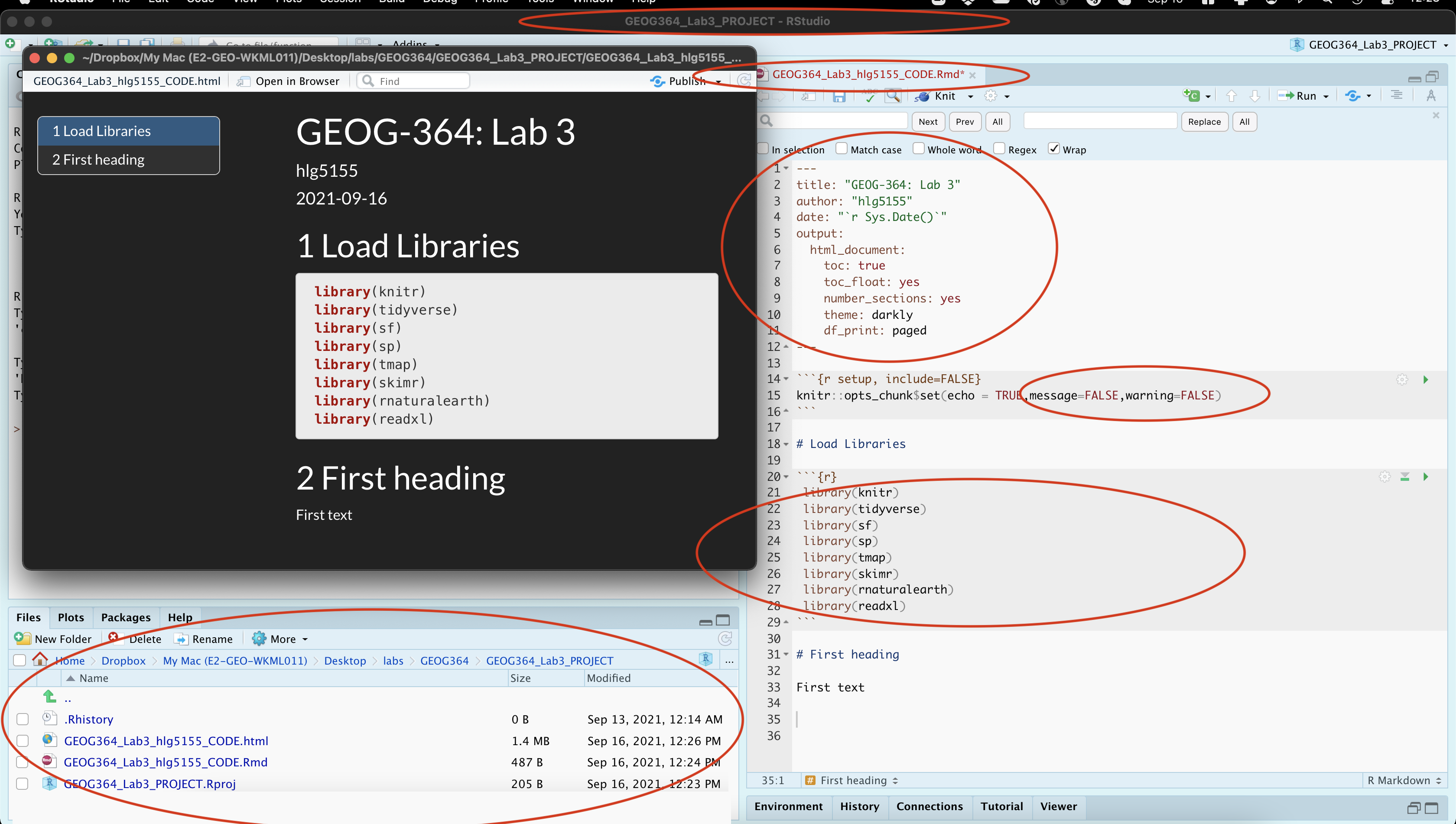
- Press knit. You screen should look like this. If so,congrats! If not, ASK FOR HELP. Note, your message=FALSE and warning = FALSE can go in the general options like my screenshot, or as “code chunk options” for the library chunk
Also, if R-studio isn’t “in” your lab 3 project, close R studio, go to your lab 3 folder and double click the .Rproj to open your lab 3 project
Step B: Commenting code
- Read Tutorial 15A: Comments to understand about code comments.
- Rename your “first heading” to “Code Comments” (or create a level 1 heading called Code Comments)
- Create a new code chunk and inside, calculate the number of characters in the word “elephant”. Write some brief comments INSIDE the code chunk to explain what you did.
Below the code chunk in the text, explain why comments might be useful.
Step C: Adding photos to text.
Reports look better with pictures & photos.
- Use Tutorial 4H to add any picture/photo of your choosing.
- In the figure caption, make sure you include the source.
Below the picture, explain why you chose it!
- Below in the text (or somewhere obvious), explain also why you added echo=FALSE into the code chunk options (hint: https://rmarkdown.rstudio.com/lesson-3.html)
Step D: Firefly analysis
Now, the lab! We are going to examine some crowd-sourced data with firefly sightings across the USA.
To to this, we are going to follow these steps. You’ll notice they are very similar to Lab 2…. (the aim of each lab is that it builds on the ones before)
- B1 Investigate the topic before touching the data
- B2 Read the file containing the data into R
- B3 Explore the “meta data” e.g. summarise the data itself
- B4 Calculate summary statistics on our columns of interest
- B5 Make the data spatial
- B6 Make some maps
D1: Exploratory Investigations
The aim of this lab is to explore spatial patterns in reported sightings of fireflies/lightning bugs. Refresh your knowledge on fireflies (these are just ideas.. spend 5-10mins on this max)
- here: https://www.massaudubon.org/learn/nature-wildlife/insects-arachnids/fireflies/about
- or this video if you’re a visual learner: https://www.youtube.com/watch?v=Y7RI1qjB2r8
- https://www.massaudubon.org/get-involved/community-science/firefly-watch/resources
Although fireflies are well loved insects, we don’t actually have a map of where they are - or if they are declining or increasing. For example, we don’t know how climate change, pesticides or light population are affecting their numbers.
To gain more data, a group of researchers started a citizen-science project called Firefly Watch where people could submit their firefly observations. See more here:
https://www.massaudubon.org/get-involved/community-science/firefly-watch
We are going to analyse some of the data from the project.
- Make a new level-1, heading called “Study Summary”
- Summarise the topic. For example, you could:
- Introduce fireflies as a topic and explain why we might want to map them
- Summarise a few facts about fireflies from your reading.
- In a new paragraph, explain the aim of the firefly watch study and how someone submits an observation.
- Make it look good! Include formatting of your choice (sub-headings, bold, bullet points, photos..).
- Introduce fireflies as a topic and explain why we might want to map them
There is a spell check next to the knit button at the top of the script. Press knit regularly to check it all looks good
D2: Read in firefly data file.
- Make a new level-1, heading called “Data Description”. Use Tutorial 6A to read the data into R and save as a variable called
firefly.
- In your read_excel code above, edit the code chunk option so that echo=FALSE and the code doesn’t show up in your final report. Tutorial 4F or (https://rmarkdown.rstudio.com/lesson-3.html)
- Now, explore the table itself and write up your results. Specifically:
- Have a look at the data using the View command (
View(firefly)), or clicking on its name - Choose some summary statistics from Tutorial 8 to assess the data (or others!).
- Have a look at the data using the View command (
- Use your analysis to answer these questions IN FULL SENTENCES in the text.
- How many observations are there? (how many rows)
- What is the unit of observation (e.g. what does each row represent?)
hint.. this is NOT one row for each firefly in the USA! See Labs/lectures for more - What variables do we have? E.g. what columns do we have for each observation?
- Which years do we have data for? How many observations in each year? (hint, apply the
table()command to the Year column of the firefly dataset) - Is Pennsylvania included in the dataset? How many observations were taken in PA?
- How many observations are there? (how many rows)
I SHOULD BE ABLE TO SEE IN YOUR CODE WHERE YOU GOT EACH ANSWER (e.g. leave your code visible)
D3: Data wrangling
- Make a new level-2, heading called “Data Wrangling”.
Read the new Tutorials on filtering and arranging data: Tutorial 7D
- Do the following tasks
- Use R to find the value of the second row and the 4th column in your data
- Filter just the rows of data that in April, and save to a new variable called april.firefly
- Use R to find the value of the second row and the 4th column in your data
- If you look closely at your summary, you might find there are some unusual temperature values.
.Let’s assume that the temperature of 8000F is not likely to be true. Filter the data so that the temperature is below 200F and overwrite (e.g. save the result as a variable called firefly).
D4: Making your data spatial
- Make a new level-1, heading called “Spatial Data”.
Read the new Tutorial on spatial data basics: Tutorial 11A
- In the text, explain why someone who has data in lat/long projection is unable to plot it with country borders in UTM Zone 17 projection.
- Read the new Tutorial 11 and 11a on creating sp data: Tutorial 11B
- In a new paragraph, explain if you think the firefly data is marked, and if so, give an example of a mark. What does the st_geometry() command do when plotting marked data?
- Your firefly data is in standard lat/lon, so EPSG=4326.
Use Tutorial 11B Make a sf version of your firefly data and assign it to a variable called firefly.sf. You can leave it in lon/lat/4326 this lab.
- Use Tutorial 11Bc to load rnaturalearth state-boundaries for US States. Assign to a variable called states.sf and use st_transform to convert to projection 4326.
D5: Making maps
Let’s now see how our data looks plotted. Create a new level-1 heading called “Data Maps”, then in a new code chunk enter the following code. You should see a basic plot with the firefly locations and the state borders. If so, congrats! If not, you need to adjust your projections or something has happened.
plot(st_geometry(firefly.sf),
pch=16,
col=rgb(0,0,1,.5),
cex=.5,
main="Firefly locations")
plot(st_geometry(states.sf),add=TRUE)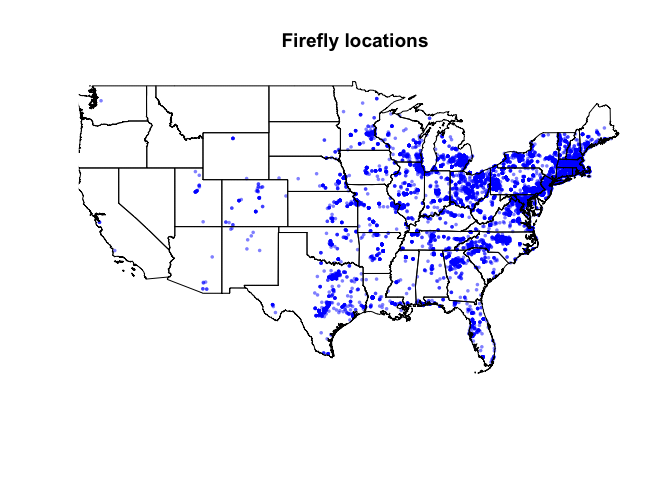
- Recreate this plot in your report. Google the
rgb()command and edit your plot so that the points are semi-transparent purple. (hint https://www.r-graph-gallery.com/43-rgb-colors.html )
The plot above is still pretty basic, so lets explore another of the big packages available to let you make “pretty plots” of spatial data. There are three big mapping functions in R: ggmap, tmap and leaflet. We’re going to look at tmap.
Look at the command below, you can see that we’re building a series of layers linked by the + symbol.
tmap_mode("plot") # Set the static plot mode
myplot <- tm_shape(firefly.sf) + # Load the firefly data
tm_dots(col="black", size=0.05) + # Plot it as dots
tm_shape(states.sf) + # Load the state borders
tm_borders(lwd=.5) # Plot them as just borders
myplot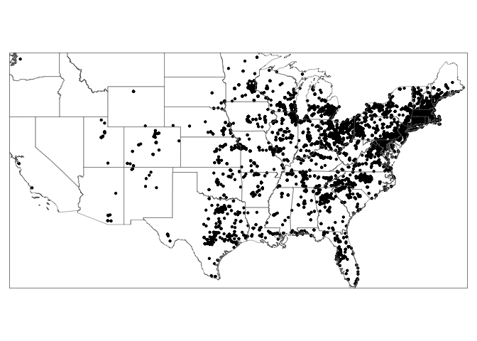
I have saved it as a variable called myplot and printed its name so that it’s saved in R. This means I can now turn on the interactive view mode and re-plot
tmap_mode("view")
myplot