Project: Dealing with Polygon Data
GEOG-364 - Spatial Analysis
Cropping data/zooming in
Required libraries
library(sp)
library(sf)
library(elevatr)
library(USAboundaries)
library(raster)
library(tidycensus)
library(rnaturalearth)
library(tmap)
library(exactextractr)
library(units)
library(tigris)
library(rmapshaper)
library(FedData)
Filtering point data sf
I am basing my examples on Iowan SVI data, SVI_county.sf
tmap_mode("plot")

tm_shape(SVI_county.sf)+
  tm_polygons("E_MOBILE",title="Estimate Living in a Mobile home/county",palette="RdPu")+
    tm_layout(legend.outside=TRUE)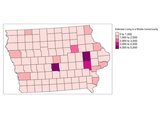
Make sure your data is in sf format! Now there are a few options. You could filter to one of the columns and crop that way. For my data I have these columns
names(SVI_county.sf)## [1] "ST" "STATE" "ST_ABBR" "COUNTY" "FIPS"
## [6] "LOCATION" "AREA_SQMI" "E_TOTPOP" "M_TOTPOP" "E_HU"
## [11] "M_HU" "E_HH" "M_HH" "E_POV" "M_POV"
## [16] "E_UNEMP" "M_UNEMP" "E_PCI" "M_PCI" "E_NOHSDP"
## [21] "M_NOHSDP" "E_AGE65" "M_AGE65" "E_AGE17" "M_AGE17"
## [26] "E_DISABL" "M_DISABL" "E_SNGPNT" "M_SNGPNT" "E_MINRTY"
## [31] "M_MINRTY" "E_LIMENG" "M_LIMENG" "E_MUNIT" "M_MUNIT"
## [36] "E_MOBILE" "M_MOBILE" "E_CROWD" "M_CROWD" "E_NOVEH"
## [41] "M_NOVEH" "E_GROUPQ" "M_GROUPQ" "EP_POV" "MP_POV"
## [46] "EP_UNEMP" "MP_UNEMP" "EP_PCI" "MP_PCI" "EP_NOHSDP"
## [51] "MP_NOHSDP" "EP_AGE65" "MP_AGE65" "EP_AGE17" "MP_AGE17"
## [56] "EP_DISABL" "MP_DISABL" "EP_SNGPNT" "MP_SNGPNT" "EP_MINRTY"
## [61] "MP_MINRTY" "EP_LIMENG" "MP_LIMENG" "EP_MUNIT" "MP_MUNIT"
## [66] "EP_MOBILE" "MP_MOBILE" "EP_CROWD" "MP_CROWD" "EP_NOVEH"
## [71] "MP_NOVEH" "EP_GROUPQ" "MP_GROUPQ" "EPL_POV" "EPL_UNEMP"
## [76] "EPL_PCI" "EPL_NOHSDP" "SPL_THEME1" "RPL_THEME1" "EPL_AGE65"
## [81] "EPL_AGE17" "EPL_DISABL" "EPL_SNGPNT" "SPL_THEME2" "RPL_THEME2"
## [86] "EPL_MINRTY" "EPL_LIMENG" "SPL_THEME3" "RPL_THEME3" "EPL_MUNIT"
## [91] "EPL_MOBILE" "EPL_CROWD" "EPL_NOVEH" "EPL_GROUPQ" "SPL_THEME4"
## [96] "RPL_THEME4" "SPL_THEMES" "RPL_THEMES" "F_POV" "F_UNEMP"
## [101] "F_PCI" "F_NOHSDP" "F_THEME1" "F_AGE65" "F_AGE17"
## [106] "F_DISABL" "F_SNGPNT" "F_THEME2" "F_MINRTY" "F_LIMENG"
## [111] "F_THEME3" "F_MUNIT" "F_MOBILE" "F_CROWD" "F_NOVEH"
## [116] "F_GROUPQ" "F_THEME4" "F_TOTAL" "E_UNINSUR" "M_UNINSUR"
## [121] "EP_UNINSUR" "MP_UNINSUR" "E_DAYPOP" "Shape_STAr" "Shape_STLe"
## [126] "geometry"So for example
#or
SVI_county.UIOWA.sf <- dplyr::filter(SVI_county.sf, COUNTY %in% c("Linn","Johnson"))

map1 <- tm_shape(SVI_county.sf)+
  tm_polygons("E_MOBILE",title="Estimate Living in a Mobile home/county",palette="Reds")+
    tm_layout(legend.outside=TRUE)


map2 <- qtm(st_geometry(SVI_county.sf))+
           tm_shape(SVI_county.UIOWA.sf)+
             tm_polygons("E_MOBILE",title="Estimate Living in a Mobile home/county",palette="Reds")+
           tm_layout(legend.outside=TRUE)


map3 <- tm_shape(SVI_county.UIOWA.sf)+
  tm_polygons("E_MOBILE",title="Estimate Living in a Mobile home/county",palette="Reds")+
    tm_layout(legend.outside=TRUE)

tmap_arrange(map1,map2,map3)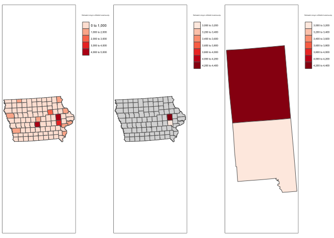
rm(map1);rm(map2); rm(map3)Cropping to a lon/lat box
Ocean folks, this one is for you!
# Make sure your sf data is in lon/lat
SVI_county.sf  <-  st_transform(SVI_county.sf,4326)

# Turn it into sp data
SVI_county.sp <- as(SVI_county.sf,"Spatial")

# My new region from https://www.geoplaner.com/
Crop.Region <- as(extent(-94,-92,41,42), "SpatialPolygons")

# Subset the polygons to my new region
SVI_county.BOX.sp <- crop(SVI_county.sp, Crop.Region, byid=TRUE)

# and convert back to sf and your other map projection
SVI_county.BOX.sf <- st_as_sf(SVI_county.BOX.sp)

SVI_county.sf  <-  st_transform(SVI_county.sf,3744)
SVI_county.BOX.sf  <-  st_transform(SVI_county.BOX.sf,3744)


# and plot -

map1 <- tm_shape(SVI_county.sf)+
             tm_polygons("E_TOTPOP",title="Estimate of the total population",
                         palette="Blues",style="log10_pretty")+
        tm_layout(legend.outside=TRUE)

map2 <- tm_shape(SVI_county.sf)+tm_borders()+
        tm_shape(SVI_county.BOX.sf)+
             tm_polygons("E_TOTPOP",title="Estimate of the total population",
                         palette="Blues",style="log10_pretty")+
        tm_layout(legend.outside=TRUE)

map3 <- tm_shape(SVI_county.BOX.sf)+
             tm_polygons("E_TOTPOP",title="Estimate of the total population",
                         palette="Blues",style="log10_pretty")+
        tm_layout(legend.outside=TRUE)

tmap_arrange(map2,map1,map3)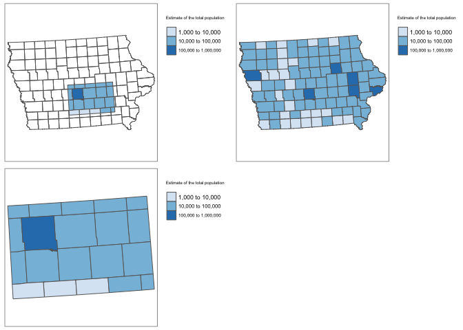
rm(map1);rm(map2);rm(map3)Cropping to a state/shapefile
Sometimes we want to crop to a state/shapefile. For example imagine we want to crop to a city metropoliton area (see Lab 7)
# This could be any sf boundary you want to crop to.
# it doesn't have to be a city - here i look for Des Moines
pl <- places(state = "IA", cb = TRUE, year=2017)
DesMoines.borders.sf <- dplyr::filter(pl, NAME == "Des Moines")

# make sure they are the same map projection
SVI_county.sf  <-  st_transform(SVI_county.sf,4326)
DesMoines.borders.sf  <-  st_transform(DesMoines.borders.sf,4326)

# and crop and save to a new thing
DesMoines.SVI.sf <- ms_clip(target = SVI_county.sf, clip = DesMoines.borders.sf, remove_slivers = TRUE)

# change the map projection back
SVI_county.sf  <-  st_transform(SVI_county.sf,3744)
DesMoines.borders.sf  <-  st_transform(DesMoines.borders.sf,3744)
DesMoines.SVI.sf  <-  st_transform(DesMoines.SVI.sf,3744)


# and plot

map1 <- qtm(st_geometry(border.county.IA.sf),fill="white")+
        tm_shape(DesMoines.SVI.sf)+
             tm_polygons("E_AGE65",title="Estimate of over 65s",
                         palette="Blues",style="log10_pretty")+
        tm_shape(DesMoines.borders.sf)+tm_borders()


map2 <- tm_shape(DesMoines.SVI.sf)+
             tm_polygons("E_AGE65",title="Estimate of over 65s",
                         palette="Blues",style="log10_pretty")+
        tm_shape(DesMoines.borders.sf)+tm_borders()

tmap_arrange(map1,map2)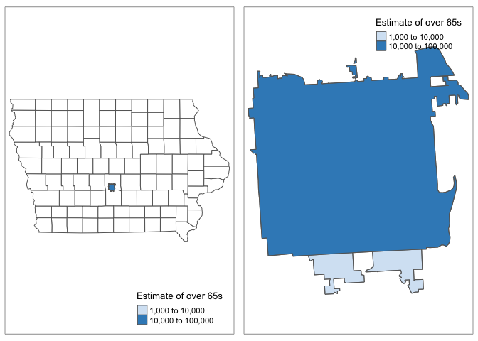
rm(map1);rm(map2)Adding in secondary data
Required libraries
library(sp)
library(sf)
library(elevatr)
library(USAboundaries)
library(raster)
library(tidycensus)
library(rnaturalearth)
library(tmap)
library(exactextractr)
library(units)
library(tigris)
library(rmapshaper)
library(FedData)
Averaging point values over polygons
There is a great tutorial here:
This is very easy using the st_join() command from the sf package. To add my census data (or any sf polygon data) to my Iowa SVI data
#--------------------------------------------------------------
# Transform all to lon/lat crs=4326 - just in case
#--------------------------------------------------------------
ACS_county.sf        <-  st_transform(ACS_county.sf,4326)
SVI_county.sf  <-  st_transform(SVI_county.sf,4326)

#--------------------------------------------------------------
# MAKE SURE THE POINT DATA GOES FIRST
# I'm calling it something new so I dont accidentally overwrite
#--------------------------------------------------------------
SVI_county.sf.all <- st_join(SVI_county.sf,ACS_county.sf)

#--------------------------------------------------------------
# Transform back
#--------------------------------------------------------------
ACS_county.sf        <-  st_transform(ACS_county.sf,3744)
SVI_county.sf  <-  st_transform(SVI_county.sf,3744)
SVI_county.sf.all <- st_transform(SVI_county.sf.all,3744)

#--------------------------------------------------------------
# and plot
#--------------------------------------------------------------
tmap_mode("plot")

map1 <- tm_shape(SVI_county.sf.all)+
             tm_polygons("E_AGE65",title="Estimate of over 65s",
                         palette="Blues",style="log10_pretty")


map2 <- tm_shape(SVI_county.sf.all)+
             tm_polygons("housevalueE",title="Estimate of house value",
                         palette="Spectral",style="log10_pretty")

tmap_arrange(map1,map2,ncol=2)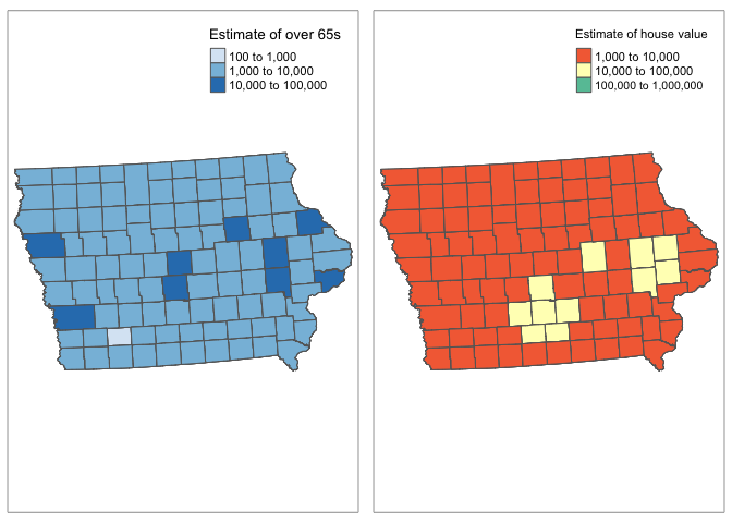
# clean up your workspace, optional but good practice unless you later need this map
rm(map2); rm(map1)
Extracting polygon values from rasters/fields
A raster is a field like elevation or land cover.
Here the elevation data is numeric whilst the land cover is categorical.
Extracting polygon values from numeric rasters
This is very easy using the exact_extract() command from the exactextractr package. To extract my elevation data
For point data, we choose simply the extract function. Remember to put results=FALSE
#--------------------------------------------------------------
# Turn everything to the same map projection
#--------------------------------------------------------------
SVI_county.sf  <-  st_transform(SVI_county.sf,crs(elevation.raster_IA))

#--------------------------------------------------------------
# add to polygon data
#--------------------------------------------------------------
SVI_county.sf$ElevationMean <- exact_extract(elevation.raster_IA,SVI_county.sf,"mean")
SVI_county.sf$ElevationMax <- exact_extract(elevation.raster_IA,SVI_county.sf,"max")
SVI_county.sf$ElevationMin <- exact_extract(elevation.raster_IA,SVI_county.sf,"min")

#--------------------------------------------------------------
# Turn everything to the final map projection
#--------------------------------------------------------------
SVI_county.sf <-  st_transform(SVI_county.sf,3744)
#--------------------------------------------------------------
# And plot
# see here for more colours: https://www.r-graph-gallery.com/38-rcolorbrewers-palettes.html
#--------------------------------------------------------------
tmap_mode("plot")
map_elev <- tm_shape(border.county.IA.sf)+
tm_polygons(alpha=0)+
tm_shape(elevation.raster_IA)+
tm_raster(title="Elevation",
palette="Spectral",style="cont",breaks=seq(100,600,100))+
tm_shape(border.county.IA.sf)+
tm_polygons(alpha=0)+
tm_layout(legend.outside = TRUE,legend.outside.position = "bottom")
map2 <- tm_shape(SVI_county.sf)+
tm_polygons("ElevationMean",title="Mean Elevation in each county",
palette="Spectral",style="cont",breaks=seq(100,600,100))+
tm_layout(legend.outside=TRUE,legend.outside.position = "bottom")
map3 <- tm_shape(SVI_county.sf)+
tm_polygons("ElevationMax",title="Max Elevation in each county",
palette="Spectral",style="cont",breaks=seq(100,600,100))+
tm_layout(legend.outside=TRUE,legend.outside.position = "bottom")
map4 <- tm_shape(SVI_county.sf)+
tm_polygons("ElevationMin",title="Min Elevation in each county",
palette="Spectral",style="cont",breaks=seq(100,600,100))+
tm_layout(legend.outside=TRUE,legend.outside.position = "bottom")
tmap_arrange(map_elev,map2,map3,map4,ncol=2)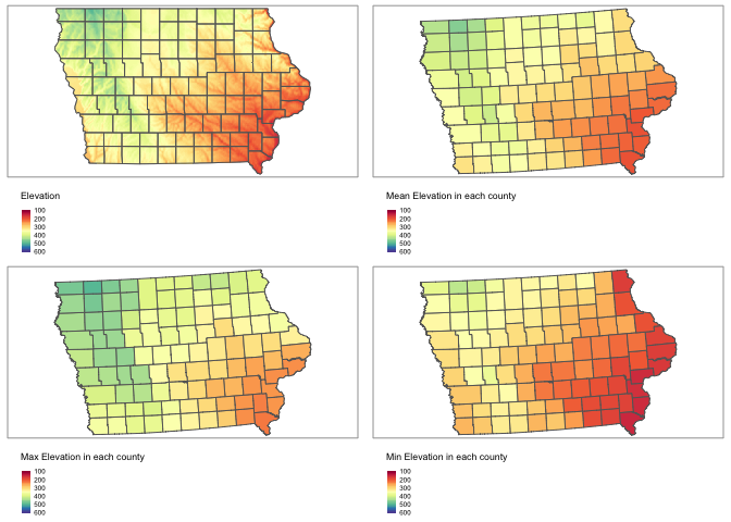
rm(map_elev); rm(map2);rm(map3);rm(map4)Extracting point values from categorical rasters
This is exactly the same but we use the “majority” function
#--------------------------------------------------------------
# Turn everything to the same map projection
#--------------------------------------------------------------
SVI_county.sf         <-  st_transform(SVI_county.sf,crs(IA_Landcover))

#--------------------------------------------------------------
# add to polygon data
#--------------------------------------------------------------
SVI_county.sf$LandcoverNumber <- exact_extract(IA_Landcover,SVI_county.sf,"majority")

#--------------------------------------------------------------
# for the landcover data specifically, this might be better
#--------------------------------------------------------------
key <- nlcd_colors()[,c("ID","Class")]
names(key) <- c("LandcoverNumber","LandcoverClass")

SVI_county.sf <- merge(SVI_county.sf ,key,by="LandcoverNumber",all.x=TRUE,all.y=FALSE)

SVI_county.sf$LandcoverNumber <- as.factor(SVI_county.sf$LandcoverNumber )
SVI_county.sf$LandcoverClass <- as.factor(SVI_county.sf$LandcoverClass )

#--------------------------------------------------------------
# Turn everything to the final map projection
#--------------------------------------------------------------
SVI_county.sf <-  st_transform(SVI_county.sf,3744)

#--------------------------------------------------------------
# And plot
# see here for more colours: https://www.r-graph-gallery.com/38-rcolorbrewers-palettes.html
#--------------------------------------------------------------
tmap_mode("plot")

map_lc1     <- tm_shape(border.county.IA.sf)+
                    tm_polygons(alpha=0)+
                tm_shape(IA_Landcover)+
                     tm_raster(title="Landcover")+
               tm_shape(border.county.IA.sf)+
                    tm_polygons(alpha=0)+
                tm_layout(legend.outside = TRUE,legend.outside.position  = "bottom")

map_lc2 <- tm_shape(SVI_county.sf)+
             tm_polygons("LandcoverNumber",title="Majority Land cover code")+
        tm_layout(legend.outside=TRUE,legend.outside.position    = "bottom")


map_lc3 <- tm_shape(SVI_county.sf)+
             tm_polygons("LandcoverClass",title="Majority Land cover class")+
        tm_layout(legend.outside=TRUE,legend.outside.position    = "bottom")


tmap_arrange(map_lc1,map_lc2,map_lc3,ncol=3)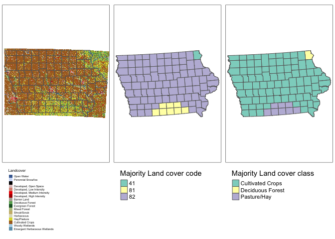
rm(map_lc1); rm(map_lc1); rm(map_lc3)