8 Regression
Now we will fit our first regression model.
8.1 “Standard” regression output
The command to do this is lm() e.g. linear model.
output <- lm(y_column ~ x_column,data=tablename)
output
NOTE, THE WEIRD ~ SYMBOL. This means “depends on”/“is modelled by” and it’s how we tell R what the response variable is. E.g. in y=mx+c, y depends on x, or y is modelled/predicted by x.
For example for the NYHouses dataset, if I wanted to create a model of the Price and Lot columns to see if Lot size could predict house sales price, then I would type.
# response = Price, predictor = Lot size
Model1.lm <- lm(Price ~ Lot,data=HousesNY)
Model1.lm
##
## Call:
## lm(formula = Price ~ Lot, data = HousesNY)
##
## Coefficients:
## (Intercept) Lot
## 114.0911 -0.5749So we are saying here that the equation is
Expected_Average_Price = -0.5749*Lot_Size + 114.0911
E.g. the average expected price house with no Lot/Garden is 114.09
8.1.1 Printing out the equation
You can also directly get the code for the model equation by the equatiomatic package
# YOU MIGHT NEED TO INSTALL THIS PACKAGE (SEE THE TUTORIAL)
library(equatiomatic)
extract_eq(Model1.lm,use_coefs=FALSE)
To make it print out directly, put “asis=TRUE” as a code chunk option e.g. this code
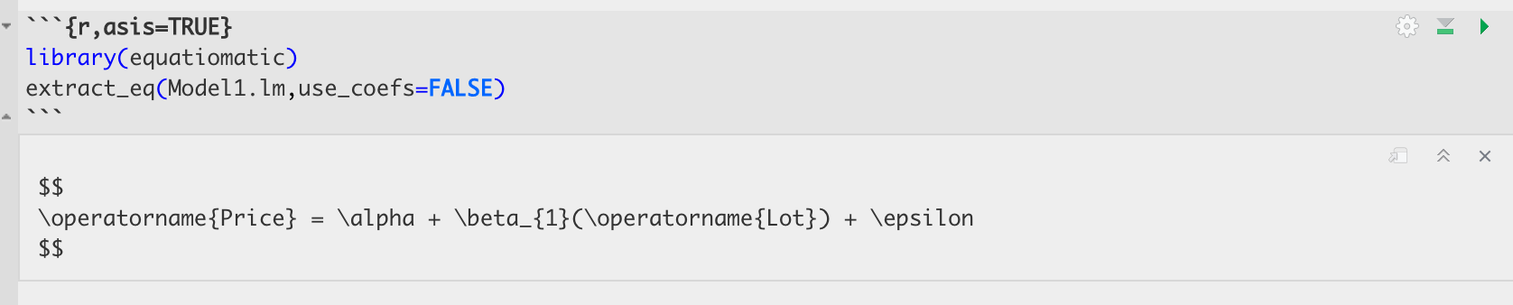
Figure 8.1: See the asis in the top, this prints the output directly when you knit
Turns into this:
library(equatiomatic)
extract_eq(Model1.lm,use_coefs=FALSE)
\[ \operatorname{Price} = \alpha + \beta_{1}(\operatorname{Lot}) + \epsilon \]
You can also look at the summary by looking at the summary command:
summary(Model1.lm)##
## Call:
## lm(formula = Price ~ Lot, data = HousesNY)
##
## Residuals:
## Min 1Q Median 3Q Max
## -74.775 -30.201 -5.941 27.070 83.984
##
## Coefficients:
## Estimate Std. Error t value Pr(>|t|)
## (Intercept) 114.0911 8.3639 13.641 <2e-16 ***
## Lot -0.5749 7.6113 -0.076 0.94
## ---
## Signif. codes: 0 '***' 0.001 '**' 0.01 '*' 0.05 '.' 0.1 ' ' 1
##
## Residual standard error: 41.83 on 51 degrees of freedom
## Multiple R-squared: 0.0001119, Adjusted R-squared: -0.01949
## F-statistic: 0.005705 on 1 and 51 DF, p-value: 0.9401In both cases, we have an estimate of the intercept (0.6386) and of the gradient (-13.8103). We will discuss the other values in later labs/lectures.
Now let’s see how to add the regression line to our scatterplot. We can do this using abline(REGRESSION_VARIABLE), where regression_variable is the name of the variable you saved the output of lm to. For example.
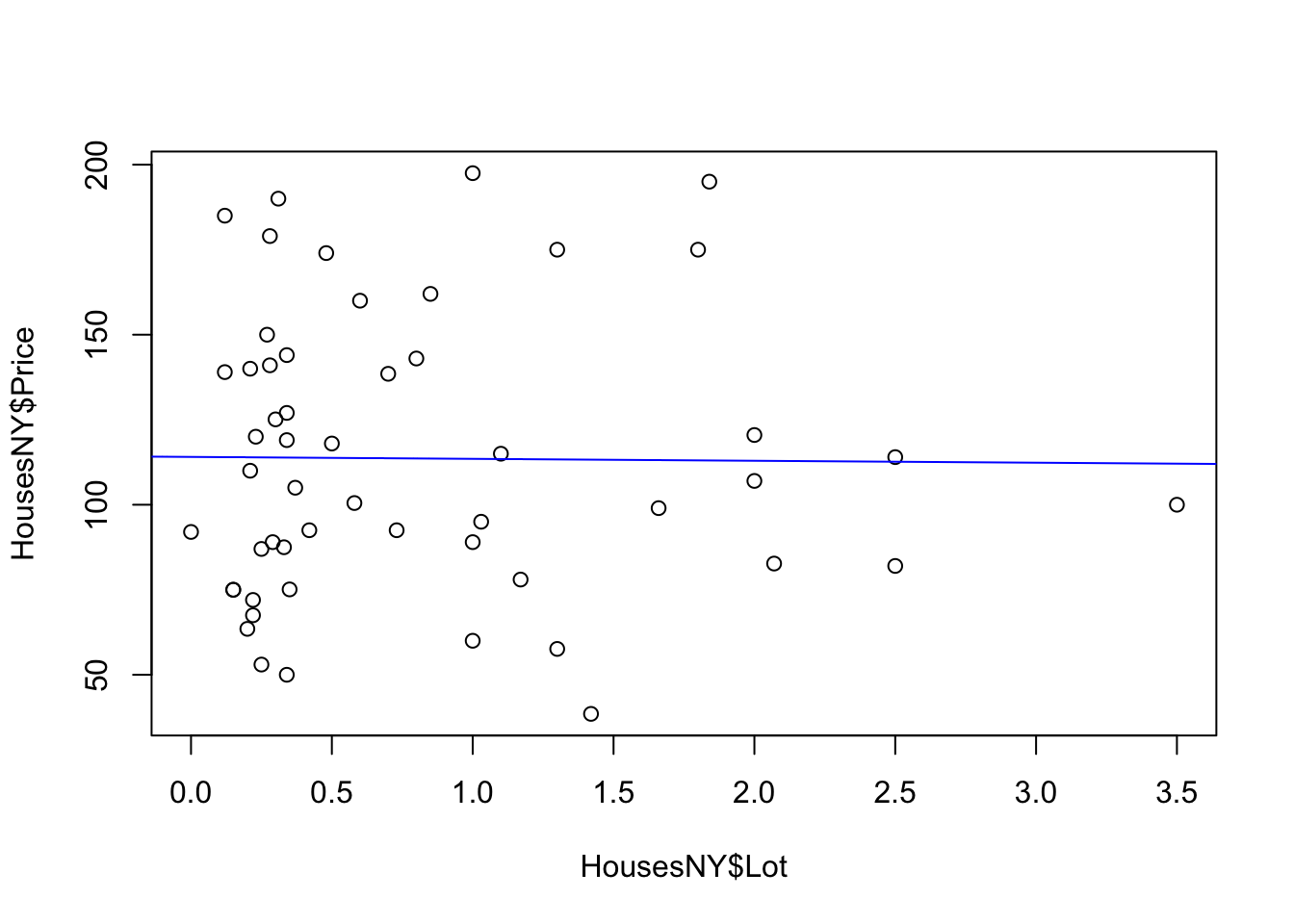
For more professional plots, see the scatterplots tutorial
8.2 “Better” OLSRR regression output
If you want a different way of seeing the same output, you can use the ols_regress() command inside the olsrr package.
library(olsrr)
Model1.lm.ols <- ols_regress(Model1.lm)
Model1.lm.ols
## Model Summary
## -----------------------------------------------------------------
## R 0.011 RMSE 41.035
## R-Squared 0.000 MSE 1749.910
## Adj. R-Squared -0.019 Coef. Var 36.813
## Pred R-Squared -0.068 AIC 550.137
## MAE 34.152 SBC 556.048
## -----------------------------------------------------------------
## RMSE: Root Mean Square Error
## MSE: Mean Square Error
## MAE: Mean Absolute Error
## AIC: Akaike Information Criteria
## SBC: Schwarz Bayesian Criteria
##
## ANOVA
## --------------------------------------------------------------------
## Sum of
## Squares DF Mean Square F Sig.
## --------------------------------------------------------------------
## Regression 9.983 1 9.983 0.006 0.9401
## Residual 89245.412 51 1749.910
## Total 89255.395 52
## --------------------------------------------------------------------
##
## Parameter Estimates
## -------------------------------------------------------------------------------------------
## model Beta Std. Error Std. Beta t Sig lower upper
## -------------------------------------------------------------------------------------------
## (Intercept) 114.091 8.364 13.641 0.000 97.300 130.882
## Lot -0.575 7.611 -0.011 -0.076 0.940 -15.855 14.705
## -------------------------------------------------------------------------------------------The ols_regress command produces beautiful output, but sometimes it doesn’t work well with other commands. So I tend to run a lm command at the same time to have both available.
8.2.1 Errors
Sometimes, this command can produce a weird error:
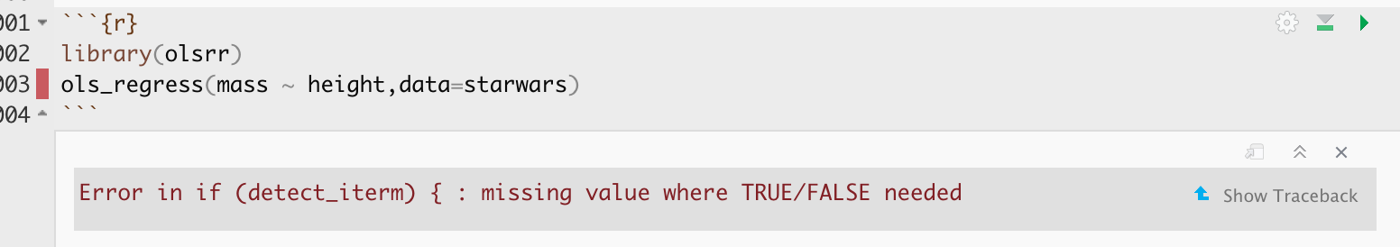
(#fig:olsrr.error)This is probably because you loaded the moderndive package
This is probably because you loaded the moderndive package. They do not play nicely together. Save your work, restart R and do not run any line that says library(moderndive)!.