Lab 4

Aim

Welcome to lab 4. This is worth 10% (100 points) and you can drop your lowest lab out of six.

By the end of this week’s lab, you will be able to:

1. Make your own .RmD report.
2. Feel comfortable reading in and filtering data
3. Feel comfortable with the core regression commands.
4. Understand in-text math equations, inline code and hidden code chunks

This is a TWO WEEK LAB. You only have two lab sessions (today and next week) working on this during class. You need to finish writing up by the following Tuesday (23:59pm) e.g. just before Lab 4 starts.

0.3.1 Need help?

REMEMBER THAT EVERY TIME YOU RE-OPEN R-STUDIO YOU NEED TO RE-RUN ALL YOUR CODE CHUNKS. The easiest way to do this is to press the “Run All” button (see the Run menu at the top right of your script)

Code won’t knit? Struggling? Have a question? See the help page here: Help!

The maximum time this lab should take is about 9-10 hrs of your time (e.g 4-5 hrs each week).

---

1. Set up (DON’T SKIP)

[Step 1.1] Create a project for Lab 4

• If you are using the POSIT Cloud (AKA R-Studio online), log-in and make a new project for lab 3 using Tutorial 1B

• If you are using R-Studio on your own computer/laptop, log in and make a new project for lab 3 using T1_ProjectsDesktop. To open/re-open your project, look in the STAT462/Lab3 folder on your computer and double click the .RProj file (I often rename it something like OPENTHIS.RProj)

[Step 1.2] Create your own lab report (NEW)

• This week you will be creating your own reports using the tutorial below, rather than downloading my template from canvas:

  • You can choose whether you want an rmdformats templates or to make/tweak your own (the tutorial link gives both options).

  • You must have a floating table of contents.

  • You must save your lab report as STAT-462_Lab4_EMAILID.Rmd** (e.g.STAT-462_Lab4_hlg5155.Rmd)

• Follow this tutorial to do this: T3_Templates

[Step 1.3] Add libraries

• Create a header-1 chapter called “Set-Up”.

  • E.g. in the text, write the word Set-Up, then using visual mode, change it to ‘header 1’ (or in source mode, write # Set-Up)

    
    

• Add a new code chunk and use this code to load the following libraries.
  
  

  • If some don’t exist on your computer or on the cloud, use Tutorial 2 to install/download them first from the app-store.
    

  • To make sure they loaded OK, run the code chunk TWICE. The second time any welcome text will disappear unless there are errors.

library(tidyverse)
library(dplyr)
library(ggpubr)
library(GGally)
library(skimr)
library(ggplot2)
library(plotly)
library(olsrr)
library(readxl)
library(yarrr)

[Step 1.4] Check Progress & knit

• You should have something like this. E.g. you are in your project, you have created your lab report and changed the author name. If you are stuck, either go back and redo the tutorials or talk to Dr G.

• Press knit and check it all works. You might need to install some packages.

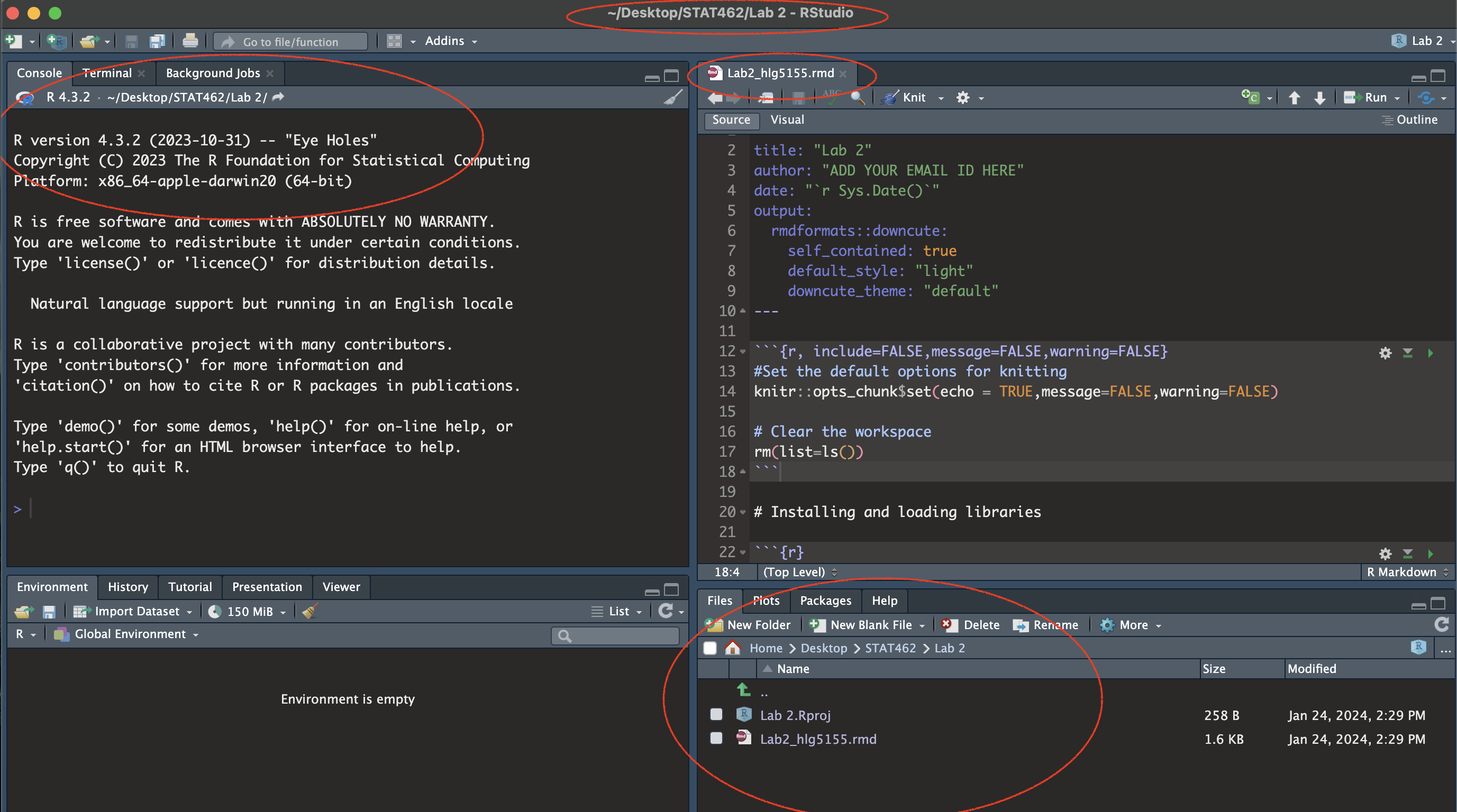
(#fig:im_Lab03_SetUp)Your screen should look like this

---

2. Challenge - Data wrangling

You are being graded in part for your style and clarity of your write up. In part this is so that it’s easier for me to grade. But by the end of the semester, I want you automatically writing reports you could show off to future employers during an interview.

So… from now onward, even if I don’t explicitly ask:

• Include your code and write up your answers as full sentences below your code.
  
  

• Include units and write up your results clearly, explaining your thinking. This is not a writing course and I am not grading you on grammar, but use the spell checker by the save button..

• For each step, make a new ‘level-2’ sub-heading. This will make the table of contents look nice.

  • In visual model you can type Step 2.1, then click on it and press Header 2.

  • In source mode you would type this, leaving a space after the ##.

      ## Step 2.1

*Note, you can type the numbers and don’t need to get R to auto-number sections,.

[Step 2]: Pirates

• Create a new level-1 heading called Pirate analysis

[Step 2.1]: Pirates data

• Load the pirates dataset from the yarrr package. (Tutorial 4.3, built in data).

[Step 2.2]: Select values

• Select the value of the pirates dataset for the 15th row and 4th column (I need to see the R code!). Write your answer as a full sentence below your r-code. Hint (Tutorial9,Wrangle basics).

[Step 2.3]: Filtering data

Hint, (Tutorial9,Wrangle basics)

• Filter the full pirates data so that it just includes pirates with more than 3 parrots and save to a new variable called pirateparrots.

• Using the table, summary, or groupby command on pirateparrots, work out the average number of tattoos of pirates with more than 3 parrots. Don’t overthink this.
  Write your answer as a full sentence below your r-code.

  
  

[Step 2.4]: Advanced Filtering

• Use similar techniques to work out how many pirates that are

  • 3+ parrot owning, male AND ALSO have more than 3 tattoos.

    
    

[Step 2.5]: Removing data

• Remove the 17th row from the main pirates dataset and overwrite (e.g. save the result to a variable called pirates)

[Step 2.6]: Combining skills

Hint, (Tutorial9,Missing data)

• In the main pirates dataset, remove the row containing the tallest pirate (let’s say the data was entered incorrectly) and overwrite.
  
  
• Now, replace the height of the shortest pirate with NA (let’s say the data was entered incorrectly) and overwrite.
  
  
• Now, use complete.cases to remove any rows where the pirate height is missing (e.g. any rows where the height is NA)

---

3. Challenge - Mystery data

• Create a new level-1 heading called Mystery Data

• Download the mystery dataset from canvas and put it into your lab 4 folder.

• Read it into R and calculate the correlation coefficient between the variables X and Y.

• Create a linear regression model between the variables X and Y.

• Write out the model equation using equation format (hint - create the equation here - https://latexeditor.lagrida.com/ , then you can put it into the text of your REPORT (not a code chunk) using double dollar signs. More in this tutorial (Tutorial3,Equations).

  $$
  YOUR EQUATION 
  $$   

  More tutorials here: https://rmd4sci.njtierney.com/math
  

• Explain why your linear model and correlation coefficient are vastly inappropriate!

  [4% total mark]

  Please work with me and don’t cheat with this question!
  Don’t tell other students the answer or even hint. or it loses the learning objective. They can still get an A* and get it wrong.

---

4. Challenge - Regression

Style

• Same as above, please write your answers as full sentences referring to your code.

• When I say a ‘professional’ plot, I mean that your axes are labelled including units and that it looks like something you might want to include in a thesis, or a report to the community group.

  • You have so many easy plot options, choose one that’s more fun than just “plot”. I often recommend the interactive plotly: (Plotly)

The problem - read carefully

Public safety spending

Suburban towns often spend a large fraction of their municipal budgets on public safety services (police, fire, and ambulance). A taxpayers’ group felt that tiny towns were likely to spend large amounts per person because they have such small financial bases. The group obtained data on the per-capita (per-person) spending on public safety for 29 suburban towns in a metropolitan area, as well as the population of each town in units of 1000 people.

They sent you the data in the file expenditure.xslx, which you can get from Canvas.

[Step 4.1]: Get the data

BEFORE you read a file into R, it is good to look at column names. It’s very frustrating in R to type column names with spaces or special characters. It makes it especially hard to refer to a column/variable by name, e.g. table$columnnamewon’t work.

You can change this in R using the names() command. But it’s much easier to fix the issue in advance. So..

• Download expenditure.xslx data from canvas and put it into your lab 4 folder.
  • If you are using posit cloud, do the steps below before uploading it.
    
• Open expenditure.xlsx in Excel and take a look!
  
  
• Rename the column titles so that no column names contains spaces/special characters & check you are happy with the data.
  
  
• Save and close, making sure that you save it to an .xlsx format.
  
  
• If you are on the posit cloud, now you can upload to your Lab 4 project.

• Create a new level-1 heading called Public Safety

• Load the data into R (Tutorial 4.2)

• In full sentences, summarize what the aim of the study is (see above), the unit of analysis, the response and predictor variables and what the taxpayer’s group expects the results to be. In your summary, assuming the taxpayer’s group is correct, write your prediction about whether the slope of Simple Linear regression model between your response and predictor should be negative or positive.

[Step 4.2]: Stacked commands

We often need to apply more than one command at once. Rather than saving the result each time and applying the next command, we can stack them together. For example, here I find the length of the longest word in the group of words

# this is the same as 
longestwordlength <- max(nchar(c("hello","cat","ice-cream")))
longestwordlength

## [1] 9

# this is the same as these commands
# where c means "stick words together"
mydata            <- c("hello","cat","ice-cream")
allwordlengths    <- nchar(mydata)
longestwordlength <- max(allwordlengths)

• Create a code chunk and calculate
  • The mean population of the sampled towns, rounded to three decimal places (hint, mean and round commands - remember you might need na.rm=TRYE)
  • The total number of towns in the sample (hint unique and length commands)

[Step 4.3]: Inline code commands

We will now learn how to hide code chunks and to automatically put the answer in your write-up.

• First, edit the code chunk options to hide the chunk when you press knit using include/echo = FALSE See (Tutorial 3, Code chunk options).

• Use inline code to write a sentence in your report telling me the number of towns in the sample and the average population of the sampled towns. See (Tutorial 3, Inline Code). THIS IS EASIER IN SOURCE MODE.

Note, if you use inline code in the future, remember to use things like ‘round’ so that your text contains an appropriate number of decimal places.

[Step 4.4]: Scatterplots

• Make a ‘professional looking scatter-plot²’ of your response and predictor WITHOUT a line of best fit. Describe it fully in the text, referring to form, direction, and strength of the association, along with the presence of any outliers.

[Step 4.5]: Regression model

• Using the data as-is, fit a regression model to the data using lm and save it as a variable called model1.

• Summarise the the model fit using OLSRR

• In the text of your report, write formally write the model equation. (hint - create the equation here - https://latexeditor.lagrida.com/ , then you can put it into the text of your REPORT (not a code chunk) using double dollar signs.

  $$
  YOUR EQUATION 
  $$   

  More tutorials here: https://rmd4sci.njtierney.com/math
  

  
  

• Create a new version of the scatterplot containing your line of best fit.

  
  

• Describe the slope and intercept within the context of the data for your community group. Explain if the slope in the output confirms the opinion of the community group?
  Explain why this initial regression might be misleading.

[Step 4.6]: Outliers

• Remove the outlier in the same way you did in challenge 2.

  
  

• Repeat the linear regression and scatter-plot with the new data and save it as a variable called model2. Explain to the community group how this has changed your assessment of the relationship between the variables.

[Step 4.7]: Correlation coefficient

Normally, to calculate the correlation coefficient between two variables, we use the cor() command or we could look at the output from ols_regress(). Let’s imagine that these have mysteriously broken.

• From only the information provided in the command summary(model2), show how you can quickly calculate the correlation coefficient and show it’s the same as the output from the model summary.
  • [HINT - HOMEWORK 5 & the Least squares derivation, just watch the video..]
  • You can use code chunks to work out the number, but explain what you are doing in the text.

[Step 4.8]: Coefficient of variation

This will be discussed in the lectures on Friday & next week, or see https://online.stat.psu.edu/stat501/lesson/1/1.5 , and https://online.stat.psu.edu/stat501/lesson/2/2.4

• Look at the ANOVA table (middle part of ols_regress(model2) or make a new code chunk and add anova(model2)).
  
  

• Using the information provided there, calculate the coefficient of variation (lecture next week)

  
  

• Explain where you can check your result in the OLSRR summary and the classic summary. E.g. upload two screenshots where you circle the result.

[Step 4.9]: Slope test

This will be discussed in the lectures next week, or see https://online.stat.psu.edu/stat501/lesson/2/2.1

• Fully write out a hypothesis test to assess of the slope is significantly different to 1.1.

  
  

• Show all your workings and professionally format any equations.
  
  

• For half marks, you can test if the slope is different to 0.

5. Submitting your Lab

Remember to save your work throughout and to spell check your writing (next to the save button). Now, press the knit button again. If you have not made any mistakes in the code then R should create a html file in your lab 4 folder which includes your answers.

For R desktop users:

• If you look at your lab 4 folder ON YOUR COMPUTER, you should see your html and Rm there - complete with a very recent time-stamp.

• In that folder, double click on the html file. This will open it in your web-browser.
  CHECK THAT THIS IS WHAT YOU WANT TO SUBMIT.

• Now go to Canvas and submit BOTH your html and your .Rmd file in Lab 4.

If you are on posit cloud,

• go to the files tab, then click the check box by your html file. Click the “more” blue cogwheel in the file quadrant menu options, then click export. This will download the file

• Uncheck the box and check the box by your .Rmd file. Click the “more” blue cogwheel in the file quadrant menu options, then click export. This will download the file.

• Now go to Canvas and submit BOTH your html and your .Rmd file in Lab 4.

Congrats! You are done.