Lab 5B

Aim

Welcome to lab 5B. This is worth 6% (60 points), alongside 40 for Lab 5A last week (you can drop them together or neither)

By the end of this lab, you will be able to:

Understand & use regression diagnostics to assess outliers
Test your knowledge on a real dataset.

This is a TWO WEEK LAB (e.g. 3 weeks total). You need to finish writing up by a week next Tuesday (Tues April 2nd 23:59pm) e.g. just before Lab 6 starts.

0.3.3 Need help?

REMEMBER THAT EVERY TIME YOU RE-OPEN R-STUDIO YOU NEED TO RE-RUN ALL YOUR CODE CHUNKS. The easiest way to do this is to press the “Run All” button (see the Run menu at the top right of your script)

Code won’t knit? Struggling? Have a question? See the help page here: Help!

The maximum time this lab should take is about 4-5 hrs of your time.

If for some reason, you didn’t do lab 5A, START THERE FIRST!

1. Set up (DON’T SKIP)

[Step 1.1] Re-Open your Lab 5 project

WE ARE CONTINUING FROM YOUR PREVIOUS LAB 5 WORK

If you are using the POSIT Cloud (AKA R-Studio online), log-in and click on your project
If you are using R-Studio on your own computer/laptop, look in the STAT462/Lab5 folder on your computer and double click the .RProj file (I often rename it something like OPENTHIS.RProj)

[Step 1.2] Re-run your previous work & check progress

You will be continuing your reports from Lab 5A.
Go to the files tab and click on the your Lab 5 .RmD lab report file to open it. (NOT THE HTML)
Go to the Session menu at the top and click “Clear Workspace”.
Now go to the session menu and click Restart R and run all code chunks. Everything in your script should run with out errors.
Press knit and check that works. Look at the html and click through your table of contents (created using those headings).
- Could you tidy up your sub-headings to make it easier to follow?
- Any spelling errors/answers that weren’t so clear?

2. Code Challenge - Regression outliers

[Step 2.1] Detecting Outliers

We will be discussing this in next week’s lectures.

FIRST, read this tutorial on identifying outliers: https://psu-spatial.github.io/Stat462-2024/T10_diagnostics.html#tests-for-outliers

Go to Canvas and download the three “testdata” datasets into your lab 5 folder (you may as well also download the bass data at this point)
Scroll to the end of your Lab report & press enter a few times. Create a level 1 heading called “Lab 5B - Outliers”
Now copy/paste this code into your report and get it running. Remember to make sure that the data is in your lab 5 folder AND you are running your project AND you have run your library code chunk.

layout(matrix(c(1,2,3), 1,3, byrow = TRUE))

testdata1 <- read_excel("testdata1.xlsx")
Model1 <- lm(y~x,data=testdata1)
plot(testdata1$y ~ testdata1$x,pch=16,xlab="x1",ylab="y1",main="Example 1") 
abline(Model1)

testdata2 <- read_excel("Testdata2.xlsx")
Model2 <- lm(y~x,data=testdata2)
plot(testdata2$y ~ testdata2$x,pch=16,xlab="x2",ylab="y2",main="Example 2") 
abline(Model2)

testdata3 <- read_excel("Testdata3.xlsx")
Model3 <- lm(y~x,data=testdata3)
plot(testdata3$y ~ testdata3$x,pch=16,xlab="x3",ylab="y3",main="Example 3") 
abline(Model3)

In your report, and using the tutorial I linked to above, describe the difference between an outlier, a high leverage point and an influential outlier.
In your report, identify which of the three Models has a high leverage point, which has an influential outlier, and which has been a non-influential outlier

[Step 2.2] Using code to detect outliers

Now run this code for each model. Below your results, explain how these plots agree/disagree with your conclusions above.

# remember to edit for model 2 and 3 
 ols_plot_resid_lev(Model1)

[Step 2.3] Understand influential outliers

Finally, this code filters out the outliers. In real life, you could use the filter command on column of your choice, remove the data in excel or use the which command. Get this running.

# remember to edit for model 2 and 3 
new_testdata1 <- testdata1[1:24,]
new_testdata2 <- testdata2[1:24,]
new_testdata3 <- testdata3[1:24,]
NewModel1 <- lm(y~x,data=new_testdata1)
NewModel2 <- lm(y~x,data=new_testdata2)
NewModel3 <- lm(y~x,data=new_testdata3)

Now examine the model slope and intercept for Model1 vs NewModel1, Model2 vs NewModel2 and Model3 vs NewModel3 (you could look at the OLSregress summary or the normal summary, or just type its name in the console). You don’t need to include all the code if you don’t want to.
In your report, use this additional evidence to explain how these plots agree/disagree with your conclusions above. Bonus, think about using the confidence intervals on the slope in the OLSRR summary to help with this.

3. Real Data - Florida Fish Challenge

[Step 3.1] Read everything in this section - you will need it!

(remember you can use google translate if/as needed)

Study Background

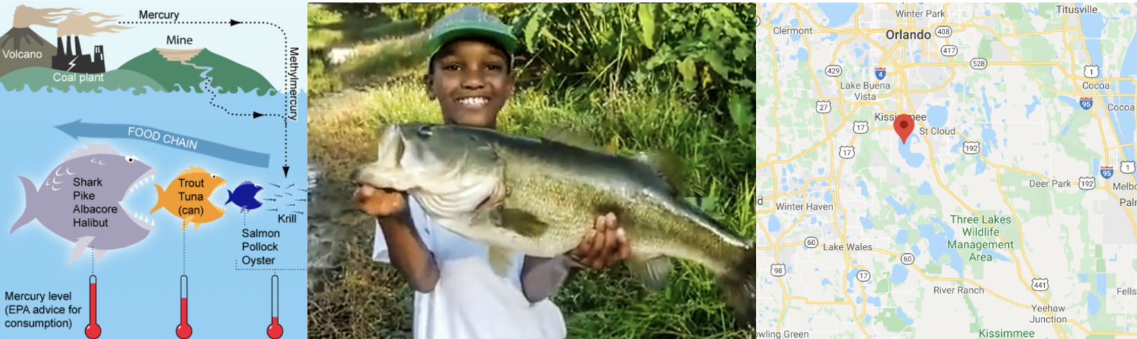
a. (Left): The mercury food chain in fish.(Wikimedia commons, Bretwood Higman, Ground Truth Trekking) b. (middle) A large bass caught and released in a central Florida lake (https://www.wired2fish.com/news/young-man-catches-releases-huge-bass-from-bank/) c. (right). The location of the lakes in Florida (Google maps)

Figure 0.1: a. (Left): The mercury food chain in fish.(Wikimedia commons, Bretwood Higman, Ground Truth Trekking) b. (middle) A large bass caught and released in a central Florida lake (https://www.wired2fish.com/news/young-man-catches-releases-huge-bass-from-bank/) c. (right). The location of the lakes in Florida (Google maps)

Small amounts of the element mercury are present in many foods. They do not normally affect your health, but too much mercury can be poisonous. Although mercury is naturally occurring, the amounts in the environment have been on the rise from industrialization. You can read more details here:

In the late 1980s, there were widespread public safety concerns in Florida about high mercury concentrations in sport fish. In 1989, the State of Florida issued an advisory urging the public to limit consumption of “top level” predatory fish from Lake Tohopekaliga and connected waters: including largemouth bass (Micropterus salmoides), bowfin (Amia calva), and gar (Lepisosteus spp.). This severely impacted tourism and the economy in the area.

Urgent research was required to inform public policy about which lakes needed to be closed. We are going to reproduce part of one study on the topic conducted by T.R. Lange in 1993.

You can see part of the paper here: https://www.researchgate.net/publication/15388314_Mercury_accumulation_in_largemouth_bass_Micropterus_salmoides_in_a\_Florida_Lake

Your Goal

You have been asked to use this dataset assess whether the alkalinity levels of a lake might impact Mercury levels in large-mouth bass.

You will be presenting your results to the Mayor of Orlando in order to set new fishing regulations.

Urgent research was required to inform public policy about which lakes needed to be closed. We are going to reproduce part of one study on the topic conducted by T.R. Lange in 1993. Dr Lange and their team took samples from 53 lakes in the Central Florida area.

Using water samples collected from each of the lakes, the researchers measured the pH level, as well as the amount of chlorophyll, calcium and alkalinity.
The Mercury concentration in the muscle tissue of lake fish was also recorded.

You can read more details in the paper/resources here - https://www.researchgate.net/publication/15388314_Mercury_accumulation_in_largemouth_bass_Micropterus_salmoides_in_a\_Florida_Lake.

The units of the your dataset are:

Variable	Unit
No_fish_sampled	Number of fish sampled from each lake
fish_av_mercury	Average amount of mercury found in sampled fish, \(\mu g\)
lake_alkalinity	miligrams/Litre, \(mg/L\) (Total alkalinity is expressed as milligrams per liter (mg/L) or parts per million (ppm) of calcium carbonate (CaCO3))
lake_ph	Unitless measure of acidity/alkalinity
lake_calcium	Measured calcium content of the lake in miligrams/Litre, \(mg/L\)
lake_chlorophyll	Measured chlorophyll content of the lake in miligrams/Litre, Micrograms, \(\mu g\)

The data is stored on Canvas in bass.xlsx.

NOTE, I HAVE CHANGED NUMBERS IN THIS DATASET - IT’S NOT THE ONE YOU SEE ONLINE..

[Step 3.2] Obtain the data

Scroll to the end of your Lab report & press enter a few times.
Create a level 1 heading called Lab 5B - Florida Fish

Obtain the data from Canvas and put it in your project folder. Use read_excel to read it into R and save it as a variable called BassNew.xlsx. e.g.

bass <- read_excel("BassNew.xlsx")

[Step 3.3] Describe the study aim

If you skipped it, go back and read the brief in 3.1. Seriously, it will save you time.
Imagine you are writing a brief for the Orlando Mayor. Start by summarizing your research goal and the data available, including
- Why people who care about Mercury poisoning are looking at fish (use the reference links)
- What you are trying to achieve in this report
- The data that is available and what population you are planning to apply it to (e.g. is your sample representative of “Florida lakes today”
- The object of analysis.
- The variables and their units (especially identifying the response variable - you’re welcome to copy/paste my table.
Use formatting like headings/sub-headings/bullet points etc to make your write up easy to read.

[Step 3.4] Exploratory analysis

Conduct a quick exploratory analysis of the data using commands like skim or summary (read ahead first!).
Below the code, in the text describe how much data is available, any missing data and any other interesting features. If you already did this above, just refer to what you did.
Make a histogram of the response variable and use any method you see fit to assess its normality. Describe your findings in the text.
Use the ggcorrmat command from the ggstatsplot package to make a correlation matrix of your bass data:
- Install the ggstatsplot package (Tutorial 2: https://psu-spatial.github.io/Stat462-2024/T2_Libraries.html#the-app-storegetting-new-packages)
- Add library(ggstatsplot) to your library code chunk
- Then at the appropriate place in your report, include

ggcorrmat(bass)

Describe the relationships you see in the text and which (if any) other predictors might be confounding variables that also impact your response variable.

[Step 3.5] First model

Create a linear model between your response and predictor (remember to read the problem statement to work out what they are). It will make your life easier to save this as a variable called model1. e.g. model1 <- ..
Make a professional looking scatterplot (this should have proper x,y axis labels etc) with the line of best fit plotted from the model. (remember https://psu-spatial.github.io/Stat462-2024/T6_plots.html#T6_PlotGGPlot)
Include the linear model summary from olsrr.
In the text below the model, formally write out the linear model equation, including the numeric coefficients.
In the text, describe the scatter-plot (e.g. strength, association, outliers etc)
The Mayor doesn’t understand statistics very well. Clearly interpret the estimated model parameters (slope & intercept)/model summary-statistics in the the context of the problem, in a way that would be understandable to a policy maker.
- By this I mean explain what the slope/intercept means in terms of fish and florida lakes, highlighting if a parameter is nonsensical (for example, knowing the weight of someone with zero height is not useful).

[Step 3.5] LINE inspection

We are now able to check for Linearity, Normality, Equal Variance and Outliers. We will look at independence in Lab 6.

Use the code from Lab 5A (at the top of your lab script!) to visually inspect
- Linearity, Equal variance and Normality of residuals (you can choose the method)
Write your conclusions in the text.

[Step 3.6] Outliers - SEE TUTORIAL 11 (NEW)

In this lab, we will now also look at Outliers. We will look at independence in Lab 6.

I have assumed that you have called your linear-model, model1 and your data, bass. Copy/edit-as-needed/run this code. This extracts from the model your predicted y-values, the residuals and outlier analysis for each data point. Get this working without errors.

# Make a new column with the predicted y value
bass$y_predicted <- model1$fitted.values

# Make a new column with the raw residuals
bass$residuals_m1 <- model1$residuals

# Make a new column with the leverage
bass$x_leverage <- ols_leverage(model1)

# Make a new column with the Cook's distance. OLSRR package
bass$cooks.distance <- cooks.distance(model1)

# Print out the table
head(bass)

Now take a look at tutorial 11 (NEW)!.

Use this data to identify:
1. The name of the lake with highest residual mercury value
2. The name of the lake with highest leverage
3. The name of the lake with highest Cook’s distance

HINT - To do this, remember you can filter and sort the data table in the View window (tiny little arrows next to each variable name) You can also use commands like max() on any column (e.g. this code would tell you the row number). Or you can sort the data using this command (https://psu-spatial.github.io/Stat462-2024/T9_wrangling.html#sorting-data)

which(tablename$columnname == max(tablename$columnname, na.rm=TRUE))

[Step 3.7] Outlier question

Another analyst looked at the scatterplot and suggested that they thought there might be three or four Lakes which appear to be either Influential, or close-to-influential outliers. If there is an outlier, then the mayor would want to send people to examine the lakes to make sure that there is nothing weird going on (which is expensive and time consuming)
In your analysis, use Cook’s distance to identify the names of lakes the analysts are worried about.
In the text explain if you agree with the comment by the analysts. Explain your reasoning and point the reader to evidence in your R output.

[Step 3.8] Transformations

Linearity appears to be the biggest problem - we are going to see if we can use a transformation to fit the data. We will cover these in next week’s lecture

To do this, we will take the log transformation of our predictor, lake_alkalinity, and save it as a new column. Full tutorial in Tutorial 13, but for now - get this running in the code:

bass$Log_Alkalinity <- log(bass$lake_alkalinity)

Now fit a NEW model between your response and lake_alkalinity (call it model2),
Plot it in a professional scatterplot (with a line of best fit)
Assess it for LINE/outliers (ignoring independence).
Write out the regression equation remembering that you are now looking at log(alkalinity) as a predictor..

Remember you can copy/paste previous code!

[Step 3.9] Model skill

Make a new sub-heading called “Model skill” to make it easy for me to find these. In your report….

Out of model 1 and model 2, discuss which model in your opinion best fits the LINE assumptions, referring to your code output above.

NOTE - QUESTION 3.9 part 2 WAS INCLUDED IN ERROR (LEFT OVER FROM AN OLD DATASET) AND HAS BEEN REMOVED.

Out of model 1 and model 2, which model explains the most variability in fish-mercury-content across the lakes?
- Provide evidence to justify your answer, including the relevant statistic for each model from your model summaries.
For model 2, are there still any outliers you might want to take a look at? Are they especially influential?
- Provide evidence to justify your answer, referring to your code above

[Step 3.10] Prediction - SEE TUTORIAL 12 (NEW)

Read Tutorial 12: https://psu-spatial.github.io/Stat462-2024/confidence-and-prediction-intervals.html

Make a new subsection called Prediction. The mayor recently had a question from a member if the public who went fishing in a new lake that was not part of the study.

We know the alkalinity level of that lake was 40mg/L.
The member of the public wants to be 99% sure that they won’t exceed the Florida Health Advisory level for Mercury levels in Fish, which is 1 \(\mu g\) of Mercury.

Should they eat the fish? You should decide the best model to use in getting to your answer.

Explain your answer and show your evidence for how you came to your conclusion.

PROBLEM SOLVING - IF YOU GOT MANY ROWS IN YOUR OUTPUT OR THE OUTPUT LOOKS STRANGE, GO BACK AND CHECK THAT YOUR LINEAR MODEL CODE IS

lm(YColumn ~ XColumn, data=mytable)

NOT

# THIS WILL BREAK THE PREDICT COMMAND LATER ON
lm(mytable$YColumn ~ mytable$XColumn, data=mytable)

See the end of Tutorial 12 for more details.

[Step 3.11] More complex - worth 3%.

Make a new subsection called Bonus.

The Florida Health Advisory level for Mercury levels in Fish is 1 \(\mu g\) of Mercury. The nayor has accepted your model and is requiring state-wide alkalinity tests.

Using your new model, what is your recommended “safety cut-off” value of alkalinity for new lakes? You would like to be 95% sure that you aren’t just seeing this result by chance. Provide evidence/code showing how you got to your answer

This question is designed to be more difficult and realistic. I will answer points of clarification, but I will not help anyone work through it before the labs are submitted. However I will award partial marks for workings and how far you get.

It is based on thinking about confidence and prediction intervals and as a hint, think about confidence and prediction intervals graphically on your scatterplot.

4. Submitting your Lab

Remember to save your work throughout and to spell check your writing (next to the save button). Now, press the knit button again. If you have not made any mistakes in the code then R should create a html file in your lab 5 folder which includes your answers.

For R desktop users:

If you look at your lab 5 folder ON YOUR COMPUTER, you should see your html and Rm there - complete with a very recent time-stamp.
In that folder, double click on the html file. This will open it in your web-browser.
CHECK THAT THIS IS WHAT YOU WANT TO SUBMIT.
Now go to Canvas and submit BOTH your html and your .Rmd file in Lab 5.

If you are on posit cloud,

go to the files tab, then click the check box by your html file. Click the “more” blue cogwheel in the file quadrant menu options, then click export. This will download the file
Uncheck the box and check the box by your .Rmd file. Click the “more” blue cogwheel in the file quadrant menu options, then click export. This will download the file.
Now go to Canvas and submit BOTH your html and your .Rmd file in Lab 5.

Congrats! You are done.

Overall, here is what your lab should correspond to:

Lab 5A

Lab 6