GEOG 364 Project Part 3
Dr Greatrex
2023-12-05
Welcome to part 3 of your projects!
The aim of this week is to continue to work on your reports (following the guidelines below), to do some point pattern analysis if you haven’t already, and add in additional datasets.
Step 0| IMPORTANT
You might find that if you have updated R, it can’t find a few packages such as sp. Remove these lines from your library code chunk - it should then run. If we get errors, Harman and I will help you through them.
The reason for this is the big R update.
Step 1| Getting started
You will be continuing with the same project folder/write up as before. So open up your project in R studio, making sure to open it by double clicking the .Rprog file on your computer (or open R studio go to “Open Project” and find your .Rproj file.
It should say your project name at the top of the screen (remember Lab 2 for how to check you are in a project).
To quickly make sure that everything is working well, go to the Session menu at the top, then click Restart R and run all chunks. This is essentially what you will do when you press knit.
Step 2| (FEEDBACK IS UP!) Reflect on feedback
Hi all, I’m very sorry that only a few of you got feedback for project 1. Know that I’m grading project stages now as they come in, so if you are running slower because of technical challenges then that is OK. If you canvas messaged me, I’m working on replying to you all.
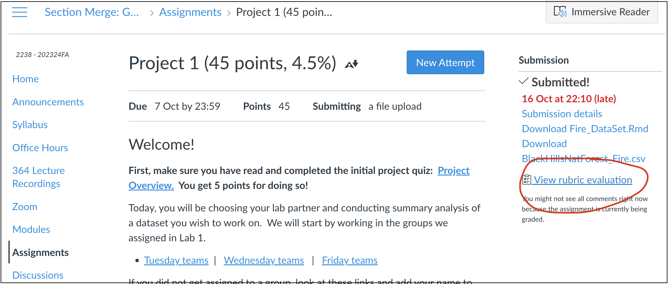
If you submitted project 2, then I have given you feedback. Go to the assignment page on Canvas and take a look at your feedback for Lab 2. See the screenshot above for where to click. https://psu.instructure.com/courses/2260204/assignments/15455259.
The most common feedback was
To keep tweaking the format e.g. put it on view mode and put in things like bullet points
To actually write your report to a person or organisation (see project 2 instructions)
To crop/filter your data to a smaller area. e.g. a single US state or X-Y box. To do this, see this tutorial https://psu-spatial.github.io/Geog364-2023/in_Tutorial06DataWrangling.html
Step 3| Check your report has everything
I have made a detailed rubric for your final report which includes everything from project 1 and 2. This is in the project menu underneath project 3.
Go and re-read your report so far and check against this rubric to make sure it has everything.
Step 4| Point Pattern Analysis
If you haven’t already, you will now conduct a point pattern analysis of your data similar to Lab 3B.
Make sure you have a UTM map projection version of your data. If you’re not sure what I mean, see here: https://psu-spatial.github.io/Geog364-2023/in_Tutorial09Spatial.html#Step_5_Assign_a_new_map_projection_ (and scroll to the top of that tutorial to read about UTM and finding your own EPSG code)
Convert the utm version of your data to the ppp format. (https://psu-spatial.github.io/Geog364-2023/in_G364_Lab3B_PointPatternDist.html#5_Convert_to_ppp_format)
Conduct the following analyses on your dataset, where you both carry out the R code AND talk about the results in your text. If you want to see an excellent example of what I mean, see this paper on earthquake damage - https://psu.instructure.com/courses/2260204/pages/reading-wartman. You don’t need to write this much! But see how they talk about the output from different techniques..
- A quadrat analysis, talking about MAUP.
- A quadrat analysis, talking about MAUP.
- Kernel density smoothing - at one or more bandwidths THAT MAKE SENSE
FOR YOUR STORY e.g. are you looking for “more in the west rather than
the east?” choose a large bandwidth. Are you looking for individual
hotspots? Choose a small bandwidth
- Kernel density smoothing - at one or more bandwidths THAT MAKE SENSE
FOR YOUR STORY e.g. are you looking for “more in the west rather than
the east?” choose a large bandwidth. Are you looking for individual
hotspots? Choose a small bandwidth
- A nearest neighbour analysis including a hypothesis test neatly
written up in the text including your H0, your H1, the test statistic,
the p-value and your interpretation (see the McGrew textbook chapter 14,
link in the point pattern lecture/lab 3A)
- A nearest neighbour analysis including a hypothesis test neatly
written up in the text including your H0, your H1, the test statistic,
the p-value and your interpretation (see the McGrew textbook chapter 14,
link in the point pattern lecture/lab 3A)
- An L-Function analysis, explained in the text
Step 4| Merging with new datasets
If you skipped here because you already did the point pattern analysis, have a look at this document - https://psu.instructure.com/courses/2260204/pages/reading-wartman . See if there are things you can add to your write up.
In the next part of the course, we will be looking at polygons and raster files. Equally R has MANY built in datasets, so I want you to be able to merge your data with new information.
Step 4A - Initial prep
Check your sf data
We will be working with the sf version of your data. To check that this hasn’t been corrupted:.
First, go to the Session menu at the very top, and click restart R and clear output. Then re-run all your code chunks.
Then, in the console, type qtm(XXXXX) where XXXXX is the sf version of your data. If it doesn’t make a map, then you have accidentally overwritten it. Ask Harman for help.
Subset to a smaller area
IF YOU HAVEN’T ALREADY, FILTER YOUR DATA TO ONE INDIVIDUAL STATE/OR X-Y BOX. You get to choose which one. You can always tweak your report reader so that they really care about one individual place..
You can do this using https://psu-spatial.github.io/Geog364-2023/in_Tutorial06DataWrangling.html.
Or if you want to crop to an X-Y box or to directly crop your sf data, see here: https://psu-spatial.github.io/Geog364-2021/364Data_TutorialWranglePoint.html#Cropping_datazooming_in
Step 4B - Read this first.
IMPORTANT - I’M TRYING TO CHECK THESE ALL FOR THE BIG SF/SP SHIFT I WAS TALKING ABOUT.
If you get weird errors, check once with Harman that it’s not a typo, send me a canvas message INCLUDING YOUR RMD FILE AND DATA, and move onto a new dataset.
When I say reading in/merging data, I mean that we will be adding information to your dataset from other sources. For example, this might be the ocean depth/temperature, the population density, the census poverty levels. You get to choose what makes sense for your reader.
You will create two things for each new dataset. The first will be a polygon or raster file for your area of interest with that new data. Secondly, you will extract the values of those fields at each of our point locations (e.g. your dataset will have a load of new columns for elevation, poverty etc).
I have included code tutorials below for many options, but you are also welcome to add in your own data (within reason). Get these easier one working before adding in your weird custom data. We won’t help you on custom data before you have done this- as it’s just a class report (maybe your report reader has weird ideas that nuclear power plants should only be placed at high elevations so you want to test this..).
For projects based in the USA, I want you to read-in/merge at least TWO other datasets.
For projects based outside the USA on land, I want you to try and read in two, but if elevation is the only one we can make work then that’s OK
For projects based in the ocean, scroll down to the ocean options
For any team looking within a sports-field, I am going to try and work on other things you can merge in, but it might be that you also read in a dataset of stadium locations for this part.
Index of tutorials
First, you might have good luck asking ChatGPT! See the first tutorial below on how I do this. Brainstorm things that your reader might be interested in looking at.
Here’s the current index of my tutorials or scroll down
Global land - Elevation
USA social data - SOVI and census data
Ocean data - Coastline and reef borders
Ocean data - Ocean Depth
Ocean data - Sea surface temperature change
USA land - Land cover/forest cover/concrete cover
Global - Weather data
Step 4C. Secondary data tutorials
Index of tutorials
Global land - Elevation
USA social data - SOVI and census data
Ocean data - Coastline and reef borders
Ocean data - Ocean Depth
Ocean data - Sea surface temperature change
USA land - Land cover/forest cover/concrete cover
Global - Weather data
Idea 0: Ask ChatGPT!
Here’s how I ask ChatGPT to do things. It’s not always right and you can rarely copy/paste, but it often provides a good guide on how to proceed.
*In R, I have point based sf data on farmers markets in iowa. I converted to utm projection using this code
IA_market.sf.utm <- st_transform(IA_market.sf,3744)
How could I automatically download elevation data for those point locations
and merge with IA_market.sf.utm? Making sure to convert everything at the end to EPSG:3744*
Or
*In R, I have point based sf data on farmers markets in iowa. I converted to utm projection using this code
IA_market.sf.utm <- st_transform(IA_market.sf,3744)
How could I automatically download land-cover data for those point locations
and merge with IA_market.sf.utm? Making sure to convert everything at the end to EPSG:3744*
If you find a package/approach no longer exists, you can repeat the
request, but add “not using the XXX package” e.g.
Or
*In R, I have point based sf data on farmers markets in iowa. I converted to utm projection using this code
IA_market.sf.utm <- st_transform(IA_market.sf,3744)
How could I automatically download land-cover data for those point locations NOT using the spData package,
and merge with IA_market.sf.utm? Making sure to convert everything at the end to EPSG:3744*
Idea 1: Elevation
Suitable for any dataset on land.
Requires the
elevatrandsfpackages. Make sure they are in your library code chunk that that it has run successfully
Read in the data
Follow this tutorial for getting it read into R. HINT, just like in Lab 4, make sure to put echo=FALSE and include=FALSE in your code chunk options when reading in this dataset. Otherwise when you press knit, your report will fill up with “downloading” output.
https://psu-spatial.github.io/Geog364-2021/364Data_TutorialDownload.html#Elevation_data note this link takes you to the 2021 lab tutorial, it will be updated ASAP, but remember come back to the 2023 page for instructions
Also note, this might require variables created higher up in the tutorial, like border files. So if you get a “this variable doesn’t exist error, use control-F to search the tutorial for that variable name and follow that earlier tutorial to create it.
Merge with your point data
Follow this tutorial for merging with your point data https://psu-spatial.github.io/Geog364-2021/364Data_TutorialWranglePoint.html#Extracting_point_values_from_rastersfields Note this link takes you to the 2021 lab tutorial, it will be updated ASAP, but remember come back to the 2023 page for instructions.
Also note, this might require variables created higher up in the tutorial, like border files. So if you get a “this variable doesn’t exist error, use control-F to search the tutorial for that variable name and follow that earlier tutorial to create it.
Update your report
Make some plots and maps! You can see my examples in the tutorial. Write about the patterns you see. You could also do things like make scatterplots between two of your variables (using plotly if you want to go interactive).
Idea 2: SOVI (from Lab 4)
Note, this also includes US Census data. There is another census package we might use later on (see here for tutorials https://crd150.github.io/lab3.html)
Suitable for any dataset in the USA which has been filtered to a single state
Requires the
elevatr,sf,tigrisandtidyversepackages. Make sure they are in your library code chunk that that it has run successfully.
Read in the data
This is fancy code that will get the SOVI data directly from the internet at census tract and county level. All you need to do is to change California to the US State of your choice and at the end, change to the map projection that matches YOUR data. You can read/talk about where the data comes from from Lab 4.
For A* candidates, see if you can understand what each line is doing and why I’m doing it.
Merge with your point data
Follow this tutorial to merge your SOVI polygon data with your UTM point data. https://psu-spatial.github.io/Geog364-2021/364Data_TutorialWranglePoint.html#Extracting_point_values_from_polygons .
Or look up internet tutorials on the st_join command. Its important that you are trying to join data in the same map projection.
Update your report
Make some plots and maps! You can see my examples in the tutorial. Write about the patterns you see. You could also do things like make scatterplots between two of your variables (using plotly if you want to go interactive).
Idea 3: OCEAN - coastline and reef border
data
Suitable for OCEAN projects. This is just border data, but it might make your maps look better.
Requires the
rnaturalearthpackages. Make sure it is in your library code chunk that that it has run successfully
Read in the data
This data comes from the rnaturalearth package, which
links automatically with the “Natural Earth” dataset, found here: https://www.naturalearthdata.com/features/ First,
download the high-resolution data in rnaturalearth by running this
command in the console. You might first need to install the remotes
package from the app store.
Now make sure that rnaturalearth is in your library code chunk and you have re-run it. This code will then allow you to get coastline and reef borders
coast.world.sf <- ne_coastline(returnclass = "sf")
reefs.world.sf <- ne_download( scale = 'large', category="physical", type = 'reefs' ,returnclass = "sf")

plot(st_geometry(reefs.world.sf),col="blue")
plot(st_geometry(coast.world.sf),add=TRUE)
Merge with your point data
You can then use st_transform to convert it to your particular map projection and see my tutorials below for how I use this to add to maps of the data
Idea 4: OCEAN Ocean depth
Suitable for OCEAN projects
Requires the
marmapandrnaturalearthpackages. Make sure they are in your library code chunk that that it has run successfully
ALL THE CODE
Follow this tutorial - https://psu-spatial.github.io/Geog364-2021/364Data_TutorialDownload.html#Ocean_floor_depth note this link takes you to the 2021 lab tutorial, it will be updated ASAP, but remember come back to the 2023 page for instructions
Also note, this might require variables created higher up in the tutorial, like border files. So if you get a “this variable doesn’t exist error, use control-F to search the tutorial for that variable name and follow that earlier tutorial to create it.
Update your report
Make some plots and maps! You can see my examples in the tutorial. Write about the patterns you see. You could also do things like make scatterplots between two of your variables (using plotly if you want to go interactive).
Idea 5: OCEAN Sea surface temperature change
Suitable for OCEAN projects
Requires the
rasterpackage. Make sure it is in your library code chunk that that it has run successfully
ALL THE CODE
Follow this tutorial - https://psu-spatial.github.io/Geog364-2021/364Data_TutorialDownload.html#Sea_Surface_Temperature_CHANGE note this link takes you to the 2021 lab tutorial, it will be updated ASAP, but remember come back to the 2023 page for instructions
Also note, this might require variables created higher up in the tutorial, like border files. So if you get a “this variable doesn’t exist error, use control-F to search the tutorial for that variable name and follow that earlier tutorial to create it.
Update your report
Make some plots and maps! You can see my examples in the tutorial. Write about the patterns you see. You could also do things like make scatterplots between two of your variables (using plotly if you want to go interactive).
Idea 6: Land Cover/Forest canopy/Concrete
Suitable for USA based projects on land
Requires the tigris and feddata packages. Make sure they are in your library code chunk that that it has run successfully
ALL THE CODE
Note, this is going to break due to the sf/sp transfer. Getting it working now, but you can always look for feddata tutorials online.
Idea 7: Weather data
Suitable for any dataset on globally. Contains global temperature/rainfall files etc.
Requires the
rasterpackage. Make sure they it is in your library code chunk that that it has run successfully
Read in the data
Follow this tutorial for getting it read into R.
https://psu-spatial.github.io/Geog364-2021/364Data_TutorialDownload.html#Weather_data note this link takes you to the 2021 lab tutorial, it will be updated ASAP, but remember come back to the 2023 page for instructions
Also note, this might require variables created higher up in the tutorial, like border files. So if you get a “this variable doesn’t exist error, use control-F to search the tutorial for that variable name and follow that earlier tutorial to create it.
Merge with your point data
Follow this tutorial for merging with your point data https://psu-spatial.github.io/Geog364-2021/364Data_TutorialDownload.html#Adding_WorldClim_to_your_datasets Note this link takes you to the 2021 lab tutorial, it will be updated ASAP, but remember come back to the 2023 page for instructions.
Also note, this might require variables created higher up in the tutorial, like border files. So if you get a “this variable doesn’t exist error, use control-F to search the tutorial for that variable name and follow that earlier tutorial to create it.
Update your report
Make some plots and maps! You can see my examples in the tutorial. Write about the patterns you see. You could also do things like make scatterplots between two of your variables (using plotly if you want to go interactive).
Submitting your report
For project three you will be graded on progress. For example, have you gotten your report closer to the final rubric, have you downloaded and merged in additional data files?