LAB IS COMPLETE

Overview

Welcome to Lab 3B on Point Pattern Analysis. The goal of Lab 3B is to learn some introductory spatial statistical approaches for characterizing distance based properties of a point pattern. We will be focusing on nearest neighbour analysis and the F, G, K and L functions. This builds on density based approaches in Lab 3A.

You need to submit everything on this page AND lab 3A under Lab 3 on canvas
See the rubric on canvas (this is up!) for how it will be graded and the checklist at the end for what you need for 100%.

See The Canvas page here, or go to canvas for assignment guidelines. You can use either the website base RStudio/Posit Cloud OR R-Desktop for this lab.

Getting stuck? Look at the canvas page for the McGrew Chapter 14 - it has a great overview.

1. What are we doing?

Density-based (Lab 3a) and distance-based (lab 3b) point pattern approaches are two different ways to analyze the spatial distribution of points or events in a dataset. They serve different purposes and provide distinct insights into the data:

density-based approaches are concerned with estimating point density and identifying areas of concentration or sparsity,
distance-based approaches focus on quantifying distances between points and using this to analyze their spatial relationships.

Each of these could capture both 1st order (changes in underlying environment) or 2nd autocorrelation (points impacting each other). In general, density tends to be more useful for situations where the underlying environment or movement of points is relatively static. Distance based approaches tend to be more useful in situations where points might move around or for 2nd order autocorrelation in general.

But choice between these approaches depends on the specific research question and the type of spatial pattern you are interested in studying.

2. Open Lab 3A

We are continuing from lab 3A with new data

Open your project for Lab 3A. Quickly reread your work and make sure that it all make sense and knits neatly. We will be continuing Lab 3B IN THE SAME DOCUMENT (e.g. you are submitting one single Lab 3 to canvas which includes both 3A and 3B).

3. Add new libraries

e.g. EDIT your existing library code chunk

We need some additional packages in lab 3B and it is good form to keep all your “library commands” at the top of your script (easier to find package related errors). Scroll up to your library code chunk at the top of your script, and add in these additional packages.

library(elevatr)
library(tidyverse)

You might need to install the packages first. If so, the easiest way is to add the library command to the code chunk, press knit/save and a little yellow banner will pop up asking if you want to install them. If it doesn’t pop-up, simply follow the instructions in Lab 3A and Tutorial 3D for installing packages.

REMEMBER DO NOT LEAVE INSTALL.PACKAGE() COMMANDS IN YOUR CODE CHUNKS. The knit button does not understand ‘go to the app store’ style commands.

Run the code chunk a few times to check for errors. Now click the Knit Button and make sure everything looks correct.

3. Read in the market data

A second element of this lab is to know how to read data into the spatstat format. This means instead of bei, you will be studying farmers markets in New York. Here I will support you directly, so you can directly copy/paste the commands into your report.

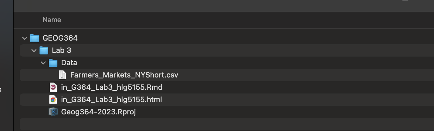
Go to the Canvas page for Lab 3 and download the file Farmers_Markets_NYShort.csv

1st, create a new heading in your report called Lab 3B farmers markets.

2nd, this first command reads in a .csv file (a basic spreadsheet - the numeric equivalent of a .txt file) and saves it as the variable market.

market     <- read.csv("./Data/Farmers_Markets_NYShort.csv")
# read.csv also works as a command. read_csv is from the tidyverse package

It doesn’t work! or There is ./Data in there I have never seen before! Do I need it???? Click here for the answer

market     <- read_csv("./Data/Farmers_Markets_NYShort.csv")

You can see in my command I have a “./Data” at the front of my address. That is because I saved my market-data inside a sub-folder called Data.

For those who have been taught setwd(), this is similar but rather than hard-wiring the location to a specific place on your computer, you are navigating within the project folder.

The “.” means “the location of the current folder” (should be your project lab folder)
The “/Data” means look inside the data sub-folder,
Then I type its EXACT name (case sensitive) including the extension.

So if your data is just in your main project folder for Lab 2, you can use its normal name as we have done before.

market     <- read_csv("Farmers_Markets_NYShort.csv")

4. Make spatial and utm

Here is how I make the data spatial (in sf format) and change the map projection.

# You can see how I try to keep everything neat with my variable names
market.sf  <- st_as_sf(market,coords=c("Longitude","Latitude"),crs=4326)

# change the map projection
market.utm <- st_transform(market.sf,crs=26918)

The first line creates an ‘sf’ version of the dataset that we can use to make maps. The coordinate column names in my data were Longitude and Latitude and the current map projection is longitude/latitude.
The second line changes the map projection from long/lat to “UTM” for the New York area.

Note, I googled the map projection I wanted to find the number (more in lab 3). I did this because the units of UTM are metres rather than degrees, a quirk that makes the spatstat package happy.

# You can see how I try to keep everything neat with my variable names
market.sf  <- st_as_sf(market,coords=c("Longitude","Latitude"),crs=4326)

# change the map projection
market.utm <- st_transform(market.sf,crs=26918)

Finally, I make a quick map of the market data to take a look:

#change to plot before knitting if you get the error 
# & restarting R annoys you
tmap_mode("view") 
qtm(market.utm)

5. Convert to ppp format

Same as last week, we will to analyse the data using commands from the spatstat package.

Just as .kml files are proprietary to Google Earth, the owners spatstat package require us to convert the data into a special format called ppp.

 # This reads the data into a ppp format, and sets the study area to the box surrounding the points.
 market.ppp <- as.ppp(market.utm)
 plot(market.ppp,use.marks = F,cex = 1, pch = 4)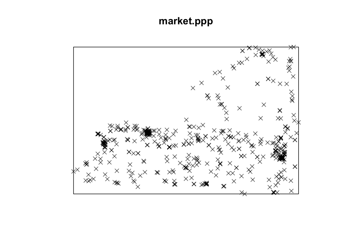

Copy the code above into a new code chunk and make sure it runs. You might get errors about Discarded datum Unknown based on GRS80 ellipsoid in CRS definition, or only first attribute column is used for marks. Ignore them.

CHALLENGE 8

You can find challenge 1-7 in Lab 3A!

Exactly follow steps 1-5 above.
The data is obtained and subset from here. https://agriculture.ny.gov/farmersmarkets . Look at this page and use it to understand the column names in your market dataset.
Use your knowledge to write a few sentences introducing farmers markets in new york (mentioning this website as the data source), what the data contains and what the column names mean.
Using the map you made and your general knowledge, write a short paragraph about the spatial patterns you see in this dataset and any 1st and 2nd order autocorrelation processes that might be behind them.

IMPORTANT - DATA NAMES

From now onward, I will continue with the longleaf data from Lab 3A.

MY longleaf example data was loaded straight from the spatstat package. It’s ALREADY a special ppp type of data.

class(longleaf)

## [1] "ppp"

But, when I read the market data into R I loaded it in as a standard table from a .csv spreadsheet.

class(market)

## [1] "spec_tbl_df" "tbl_df"      "tbl"         "data.frame"

To convert it to spatial, we made sf-longlat, sf-utm and ppp versions of the market data (in order to do specific things in those packages). I wanted a way to keep track. So I edited the names to include a .ppp, a .sf and a .utm e.g. I decided the name of my ppp market data would be market.ppp

But I COULD have called them anything

# These are EXACTLY the same, I just saved them as different names
 market.ppp  <- as.ppp(market.utm)
 catsarecool <- as.ppp(market.utm)
 
 class(market.ppp)

## [1] "ppp"

 class(catsarecool)

## [1] "ppp"

So in your next section, I will use “longleaf” as my input. You will use market.ppp as your input E.g.

# Again, I can name the OUTPUT whatever I want! 
# But the input needs to have already been created 
# and be the correct variable type

mysummarylooooongleaf   <- summary(longleaf)
mysummarymarket         <- summary(market.ppp)

If you accidentally put market.ppp as your output e.g.

market.ppp <- 5

Then you will overwrite it! It will no longer be a special ppp table, it will be the number 5. Then the rest of your code won’t work.

6. Nearest neighbour plots

The nndist command calculates the distance of the nearest neighbour for every point. Going back to my longleaf data from Lab 3A, here is what I would type:

# Nearest neighbour analysis
# Hint, your ppp variable for the INPUT is called *market.ppp*.  
# Mine is called longleaf. 
# The command is nndist
# I saved my output as a custom name, longleaf_nnd 
# e.g. longleaf nearest neighbour. You can call yours anything you like
 
longleaf_nnd <- nndist(longleaf)

#now I make a histogram of nearest neighbours
 hist(longleaf_nnd,br=50)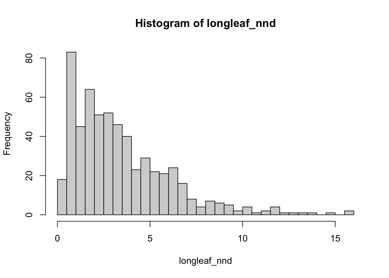

In the first line, - the COMMAND is nndist (so if I wanted I could look at its help file), - I apply the command to my longleaf variable - and I save the answer to a new variable called longleaf.nnd (e.g. the longleaf nearest neighbour distances)

7. Average nearest neighbour

We can now easily calculate the average nearest neighbor distance using the mean command. Here is how I stack commands to make a prettier output, using paste and “c” to stick things together.

# Mean nearest neighbour
#-------------------------------------
 paste( c("The average nearest neighbour of my longleaf data is:"),
        round(mean(longleaf_nnd),3),"m away")

## [1] "The average nearest neighbour of my longleaf data is: 3.443 m away"

This is exactly the same as

# find single observed average distance for the whole field.
longleaf.obs_mean_nnd  <- mean(longleaf_nnd) 
# round the answer to 3 decimal places
round.longleaf.obs_mean_nnd <-  round(longleaf.obs_mean_nnd,3)

# make my answer
print("The average nearest neighbour of my longleaf data is:")

## [1] "The average nearest neighbour of my longleaf data is:"

round.longleaf.obs_mean_nnd

## [1] 3.443

print("m away")

## [1] "m away"

8. Clarke-Evans Ratio, R

This ratio is named after the people who invented it, Clarke & Evans. Type ?clarkevans into the help file for more details and look at the textbook/google point pattern clarke evans ratio for more information.

I can create these and print them out using the following commands, again I am making my code look neater.

# R ratio applied to the ppp variable itself, yours is called market.ppp
#----------------------------------
 longleaf.obs.RRatio <- clarkevans(longleaf)
 longleaf.obs.RRatio

The output of the R.Ratio likely gives you two values, naive and cdf. CDF is simply a mathematical way of taking into account edge effects, more details here: https://www.jstor.org/stable/20146996

So in this case, R= 0.832 - showing slightly clustered data.

It doesn’t work! I get an error! Click here for the answer

If your error is this,

then look upwards in your code for the last time you typed market.ppp.

Did you accidentally save it as an OUTPUT (e.g. market.ppp <- …..)?

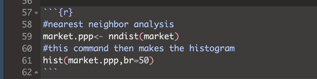
If so, go back and re-read that “IMPORTANT DATA NAME SECTION” because probably you have overwritten it with something else! It might be called .ppp, but its contents are no longer a ppp type. For example, this line will run without error in its own right, but in running it, you overwrote your ppp answer with a list of nearest neighbour distances. So now, nothing in the future that needs the actual ppp data will work.

# you applied the command nndist to the variable market, then overwrote your existing ppp variable with the answer 
market.ppp<- nndist(market)

Go back, change it and re-run all your code chunks!

9. Clarke-Evans hypothesis test

Finally, we can conduct a hypothesis test on the ratio output:

clarkevans.test(longleaf)

## 
##  Clark-Evans test
##  Donnelly correction
##  Z-test
## 
## data:  longleaf
## R = 0.81768, p-value < 2.2e-16
## alternative hypothesis: two-sided

If we look at the help file (?clarkevans.test), we can see

H0: The pattern shows complete spatial randomness caused by an independent random process. R=1. E.g. If we simulated 100 random point patterns and calculated the Clarke Evans ratio for each, we would get a histogram with a mean of 1.
H1: The pattern is unusually DIFFERENT (e.g. strangely clustered OR strangely uniform) compared to what we would expect in H0. E.g. R would be high or low.

From the R output, the observed R was 0.83. A randomly created H0 pattern would only expect to see something like this once every 1000,000,000,000,000 times. It’s a very unusual result (e.g. the probability of seeing it is tiny).

Therefore I personally have enough evidence to reject the null hypothesis and say a random independent process probably isn’t causing the autocorrelation pattern of longleaf trees in my study area.

CHALLENGE 9

Create a new heading called nearest neighbour *(spelled either the American or British way..)*
Get the code in tutorials 6-9 working for your market data
- IF YOU GET ERRORS RE-READ THE IMPORTANT DATA NAME & “I GOT AN ERROR” BITS
Explain what the output of the code is showing you for the nearest neighbour and Clarke Evans Ratio for farmers markets in New York. What units are the distances in? (hint, google the units of your new map projection)
1. Bonus - add another layer in my fancy stacked code to convert to km using basic maths.
Now write your interpretation of the output.
#
- What would the clarke evens ratio, R, be for very disperse data?
- What would the clarke evens ratio, R, be for very clustered data?
- Does this show whether NY farmers markets are clustered, random or dispersed?
Conduct a ONE-SIDED clarke evans hypothesis test on whether your market data is more CLUSTERED than you expect and interpret the result (hint go back to the Canvas page for the textbook chapter 14 and the clarkeevans.text help file for modifying the code).
Write a short paragraph for each of the following
1. What are edge effects in point pattern data? Are they going be an issue for this SPECIFIC dataset/analysis and why?
2. What is the locational fallacy? Is it going going be an issue for this SPECIFIC dataset/analysis and why?
3. What is MAUP? Is it going be an issue for this SPECIFIC dataset/analysis and why?

10. Ripley’s L-Function

We will now conduct an L-Function analysis on the data. This is a version of Ripley’s K that is easier to interpret. This code won’t show any output if it runs correctly because I’ve saved all the outputs to variables.

Note, my variable names are long in this class to stay informative

# Calculate the L function. Your data is market.ppp
longleaf.lest <- Lest(longleaf,correction = "Ripley")

# Create an ensemble (collection) of simulated point patterns 
# that is based on our data data, 
# but the points have been rearranged using an independent random process. 
# For each one, calculate the L function, lest
# 
longleaf.lest.IRPsimulation <- envelope(longleaf, 
                              Lest, correction = "Ripley", 
                              verbose = F,
                              nsim=100, nrank=1, 
                              savepatterns = FALSE, savefuns = FALSE)

Now we can plot the data. This command is horrible, just copy/paste changing longleaf to your market data. I will look for a better one!

#Find the max and min values
L.EST.Max<-(max(longleaf.lest$iso-longleaf.lest$r))
L.EST.Min <- 0-L.EST.Max

#The dots are weirdly important here. Copy/paste
plot(longleaf.lest,. - r ~ r, ylim=c(L.EST.Min,L.EST.Max))

# Add IRP simulated Lestimates (so many, they merge into a grey cloud)
plot(longleaf.lest.IRPsimulation, . - r ~ r,add=TRUE)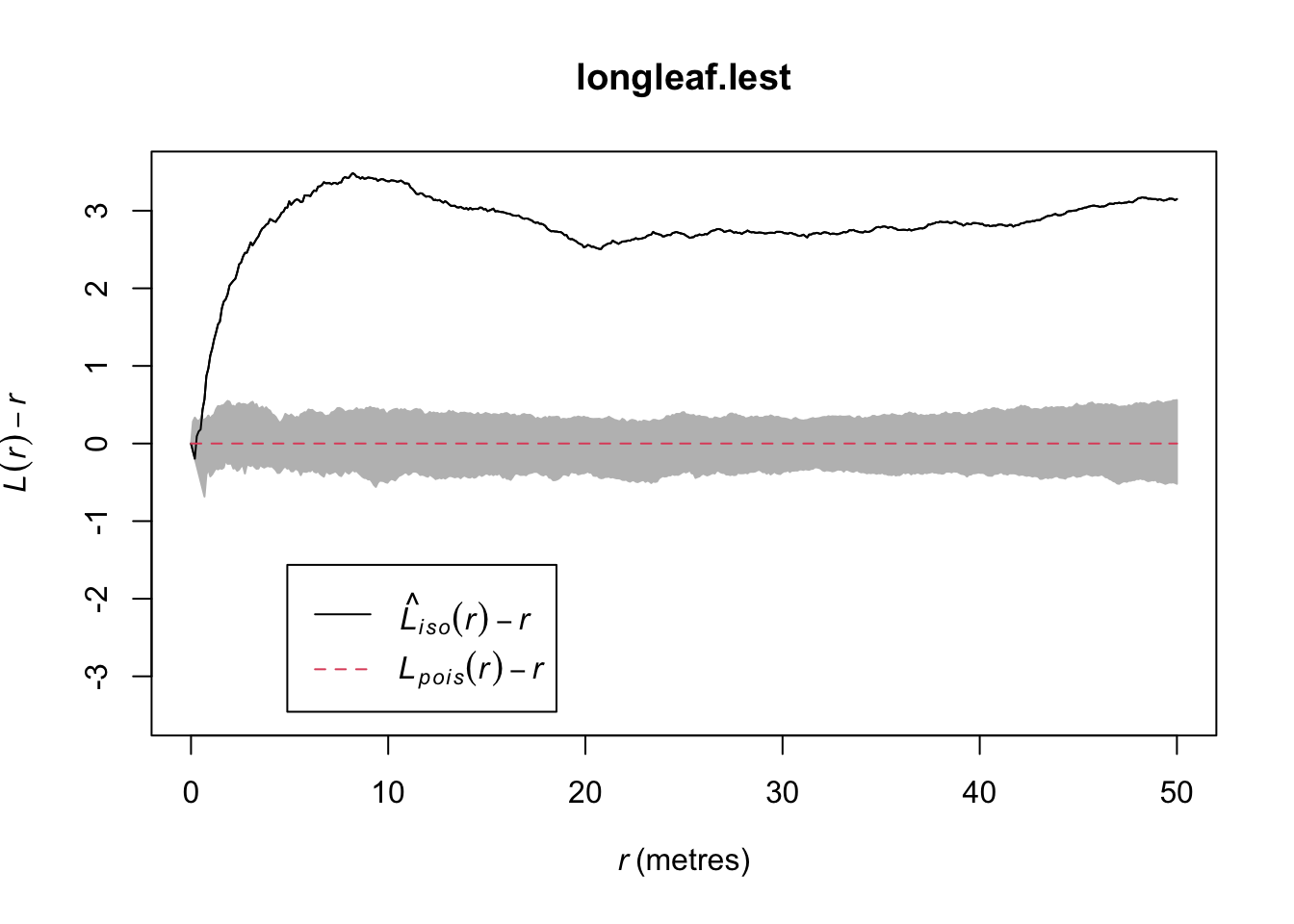

We will talk about the interpretation in class. But simply, the data is unusually clustered (above the grey cloud) at all scales.

CHALLENGE 10

Get the L-function code working on your market data. You will find that the grey cloud does not show up!
Play with the number of simulations (nsim) and re-run the two code chunks. (e.g. set it to 10 and re-run, set it to 1000 and rerun) Why does the grey cloud get larger as the number of simulations increases?
Interpret the output of your L-Function in the text. Because H0: CSR is a boring comparison, this will be pretty clear. In class I will show you how to get more complex.
Look at the help file for the Kest command (easier to read) and explain what the “correction” option is doing. What are some of the other options available?

LAB IS COMPLETE

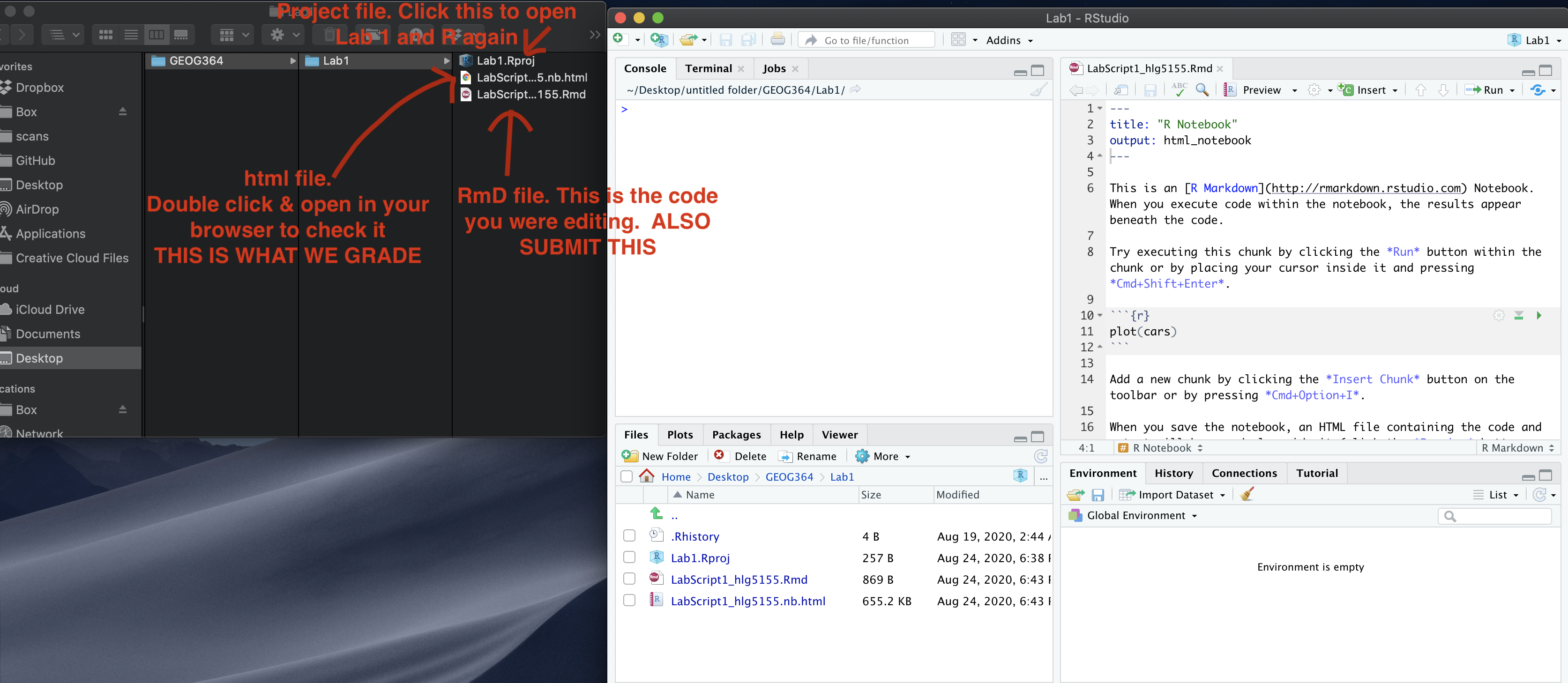
Submitting your work

Remember to save your work throughout and to spell check! (next to the save button). Now, press the knit button one final time.

On R-Desktop

If you have not made any mistakes in the code then R should create a html file in your lab 3 folder which includes your answers.
If you look at your lab 3 folder on your computer, you should see the html there - complete with a very recent time-stamp. Double click on the html file. This will open it in your web-browser.
CHECK THAT THIS IS WHAT YOU WANT TO SUBMIT.

On Rstudio cloud,

See TUTORIAL 3 Cloud - LINK FIXED for how to download your files

Finally, go to Canvas and submit BOTH your html and your .Rmd file in Lab 3.

How am I graded?

Overall, here is what your lab should correspond to:

POINTS	Approx grade	What it means
98-100	A*	Exceptional. Above and beyond. THIS IS HARD TO GET.
93-98	A	Everything asked for with high quality. Class example
85-93	B+/A-	Solid work but the odd mistake or missing answer in either the code or interpretation
70-85	B-/B	Starting to miss entire/questions sections, or multiple larger mistakes. Still a solid attempt.
60-70	C/C+	It’s clear you tried and learned something. Just attending labs will get you this much as we can help you get to this stage
40-60	D	You submit a single word AND have reached out to Dr G or Aish for help before the deadline (make sure to comment you did this so we can check)
30-40	F	You submit a single word……. ANYTHING.. Think, that’s 30-40 marks towards your total….
0+	F	Didn’t submit, or incredibly limited attempt.

Lab 3B: Point Pattern Distance

Lab 3 is split into two parts to match the lectures

LAB IS COMPLETE

Overview

1. What are we doing?

2. Open Lab 3A

3. Add new libraries

3. Read in the market data

4. Make spatial and utm

5. Convert to ppp format

CHALLENGE 8

IMPORTANT - DATA NAMES

6. Nearest neighbour plots

7. Average nearest neighbour

8. Clarke-Evans Ratio, R

9. Clarke-Evans hypothesis test

CHALLENGE 9

10. Ripley’s L-Function

CHALLENGE 10

LAB IS COMPLETE

Submitting your work

How am I graded?