Lab 5: Moran and Lisa
One week lab!
One week lab!
1. Welcome to Lab 5
The objective of this lab is to introduce you to the concept of Moran’s I and LISA.
This is due by 23:59pm Sunday 10th December.
See the rubric on canvas for how it will be graded and the checklist
at the end for what you need for 100%.
2. Important (please read!)
We are continuing to focus on air pollution in California and build on Lab 4.
You can read about the data and remind yourself of things like column names from the description of Lab 4.
But! Due to the challenges facing those using R studio cloud, I have created spatial data files of all the processed data from lab 4 and I have included much of the code for lab 5.
THIS MEANS WE WILL BE CREATING A COMPLETELY NEW LAB PROJECT AS THOUGH IT WAS A NEW TOPIC (See below for instructions).
3. Getting started.
A. Create your project
In Desktop R, select your 364 directory, create a new project, then name the project Lab 5. If you are stuck on this process, see these tutorials
For R-Desktop, see Tutorial 3B
For Posit Cloud, see Tutorial 3C
You can check this has worked by looking on the file explorer on your
computer, then selecting your GEOG364 folder and checking that a Lab 5
folder has appeared with your .Proj file inside it. This is
what you double click to access this lab in R.
4. Get the lab report template and data
Go to CANVAS LAB 5, download the lab report template and all the data sets. If you are on the cloud, ignore the census tract dataset. Rename the lab report (the .RmD file) to include your email ID and place EVERYTHING in your Lab 5 folder.
Now open your project and your lab report template (the .RmD file).
5. Complete the lab report
I have included all of these instructions in the lab report itself, but it will make life easier to read them first here so you know what you are doing.
A. Read in the data
Get Section A of your lab script running and make sure it has read in the data without error. Talk to a teacher if you have any issues (and make sure the data is in the same folder as your .proj file and not accidentally in a sub-folder or a different place)
B. Voronoi polygons
In Section B of your report, I have provided some code which summarizes and maps the ozone data by counties and voronoi polygons. You should be able to just run the code and it will make the plots
In your report, below the code:
Describe what each map is showing and what voronoi polygons are.
Compare and contrast the three maps.
For each map, explain the advantages and disadvantages of using this way to summarize & visualize the ozone data.
C. Moran’s I tutorial
There is an excellent tutorial on Moran’s I created by Dr Manny Gimond here on incomes in Maine. We will also be working through this in class.
https://mgimond.github.io/simple_moransI_example/
In Section C (‘Maine Tutorial’) of your lab report, I want you to
work through the tutorial. (You do not have to do the Florida homicides
bit).
- I want the code working in your lab report,
- I also want as many comments as you can following along in the text,
e.g. make yourself a tutorial IN YOUR OWN WORDS
D. Moran’s I of the California data
In Section D of your lab report, I provided a shortened version of the code in Dr Gimond’s tutorial. My code is set to look at the ozone levels. Get it running, then in your report under my code, interpret what I found in your own words.
Then, copy and edit my code to conduct a Moran’s I analysis of a variable (column) of your choice and interpret your findings in the text.
E. LISA analysis
Finally, my code for the LISA analysis should just run. Using the lecture notes and readings interpret what the maps are showing you. Your write up should include
- What do each of the four colors/quadrants mean
- How do they link to the Moran scatterplot
- Change the critical value to 0.01, and to 0.1 and to 0.5 - and each
time, re-run the LISA code (everything below the critical value).
Explain what is happening in terms of ozone pollution in California.
6. Submitting your work
Remember to save your work throughout and to spell check! (next to the save button). Now, press the knit button one final time.
On R-Desktop
If you have not made any mistakes in the code then R should create a html file in your lab 5 folder which includes your answers.
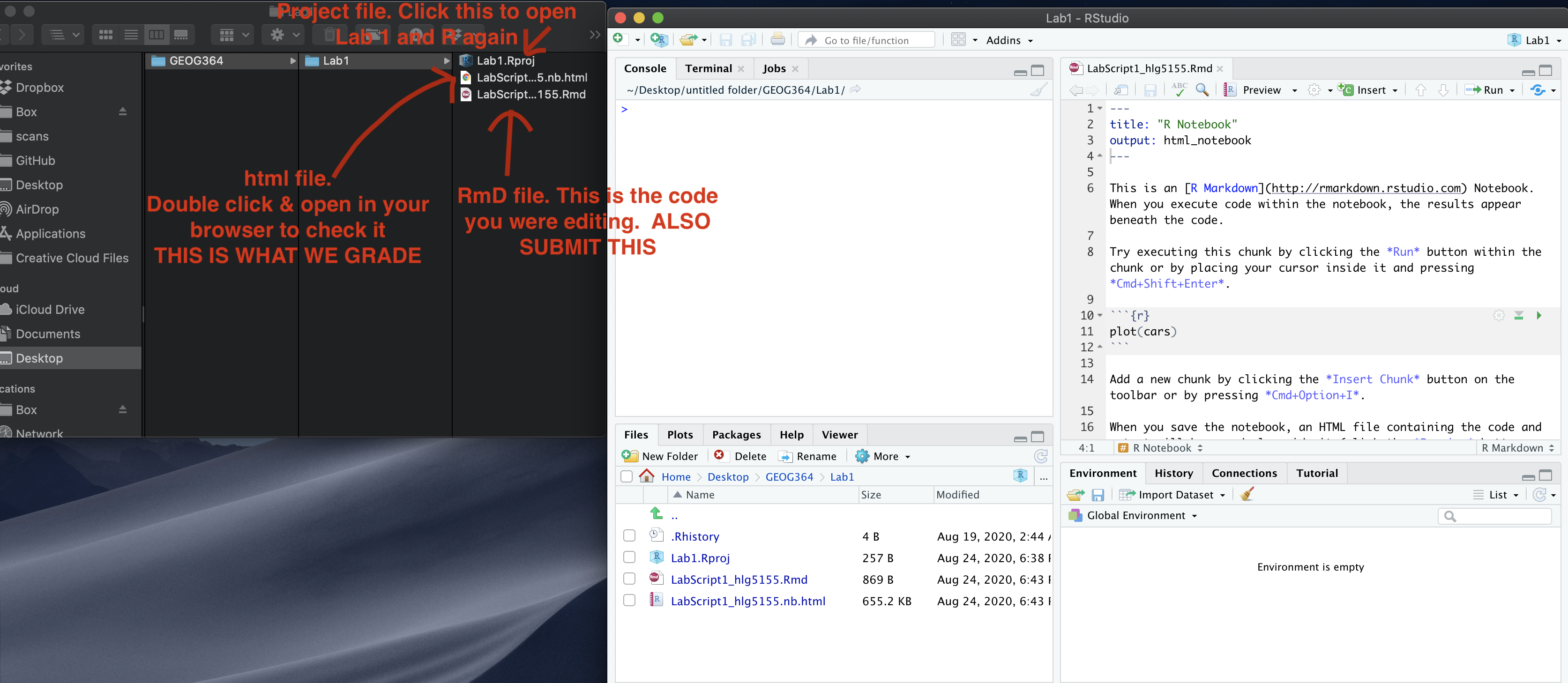
If you look at your lab 5 folder on your computer, you should see the html there - complete with a very recent time-stamp. Double click on the html file. This will open it in your web-browser.
CHECK THAT THIS IS WHAT YOU WANT TO SUBMIT.
On Rstudio cloud,
- See TUTORIAL
3 Cloud - LINK FIXED for how to download your files
Finally, go to Canvas and submit BOTH your html and your .Rmd file in Lab 3.
How am I graded?
Overall, here is what your lab should correspond to:
| POINTS | Approx grade | What it means |
|---|---|---|
| 98-100 | A* | Exceptional. Above and beyond. THIS IS HARD TO GET. |
| 93-98 | A | Everything asked for with high quality. Class example |
| 85-93 | B+/A- | Solid work but the odd mistake or missing answer in either the code or interpretation |
| 70-85 | B-/B | Starting to miss entire/questions sections, or multiple larger mistakes. Still a solid attempt. |
| 60-70 | C/C+ | It’s clear you tried and learned something. Just attending labs will get you this much as we can help you get to this stage |
| 40-60 | D | You submit a single word AND have reached out to Dr G or Aish for help before the deadline (make sure to comment you did this so we can check) |
| 30-40 | F | You submit a single word……. ANYTHING.. Think, that’s 30-40 marks towards your total…. |
| 0+ | F | Didn’t submit, or incredibly limited attempt. |