1 Main report: Seoul Bike Rental Analysis
1.1 Study background
Bike rentals are an important transportation options in many urban areas. For a bike sharing programme to be a success, it is important to understand what impacts demand, so that rental bikes are available and accessible to the public at the right time and place. This could enbable a city to have a better supply of rental bikes.
My client is the manager of the Seoul Bike Sharing programme in South Korea. They have asked me to assess the data they have collected to understand how to model demand.
1.2 Dataset description
The data my client provided is a subset of a larger dataset accessible here: https://archive.ics.uci.edu/ml/datasets/Seoul+Bike+Sharing+Demand. The data originally collected through the Seoul Open Data project/ http://data.seoul.go.kr/.
The data has 8760 observations, where each observation is an hour of an individual day. For each hour, the following data was collected:
- Date : year-month-day (Date)
- Rented Bike count - Count of bikes rented at each hour in the Seoul bike rental system (Count data)
- Hour - Hour of the day (integer)
- Temperature - in Celsius (numeric continuous)
- Humidity - % (numeric continuous)
- Windspeed - m/s (numeric continuous)
- Visibility - 10m (numeric continuous)
- Dew point temperature - Celsius (numeric continuous)
- Solar radiation - MJ/m2 (numeric continuous)
- Rainfall - mm (numeric continuous)
- Snowfall - cm (numeric continuous)
- Seasons - Winter, Spring, Summer, Autumn (categorical ordinal)
- Holiday - Holiday/No holiday (categorical nominal)
Unfortunately in the dataset provided to me, it appears that the Date column was lost. Equally, there is very little information about how the data was collected, or about the population. For example, I could imagine that the number of bike rentals might change over time as the programme grows or shrinks, but I do not have informaiton to take this formally into account.
The summary statistics for the dataset can be seen below. There is no missing data in the dataset.
| Name | bike |
| Number of rows | 8760 |
| Number of columns | 11 |
| _______________________ | |
| Column type frequency: | |
| factor | 2 |
| numeric | 9 |
| ________________________ | |
| Group variables | None |
Variable type: factor
| skim_variable | n_missing | complete_rate | ordered | n_unique | top_counts |
|---|---|---|---|---|---|
| Season | 0 | 1 | FALSE | 4 | Spr: 2208, Sum: 2208, Aut: 2184, Win: 2160 |
| Holiday | 0 | 1 | FALSE | 2 | No : 8328, Hol: 432 |
Variable type: numeric
| skim_variable | n_missing | complete_rate | mean | sd | p0 | p25 | p50 | p75 | p100 | hist |
|---|---|---|---|---|---|---|---|---|---|---|
| Rental.Count | 0 | 1 | 704.60 | 645.00 | 0.0 | 191.00 | 504.50 | 1065.25 | 3556.00 | ▇▃▂▁▁ |
| Hour | 0 | 1 | 11.50 | 6.92 | 0.0 | 5.75 | 11.50 | 17.25 | 23.00 | ▇▇▆▇▇ |
| Temperature | 0 | 1 | 12.88 | 11.94 | -17.8 | 3.50 | 13.70 | 22.50 | 39.40 | ▂▆▆▇▂ |
| Humidity | 0 | 1 | 58.23 | 20.36 | 0.0 | 42.00 | 57.00 | 74.00 | 98.00 | ▁▅▇▇▅ |
| Wind.Speed | 0 | 1 | 1.72 | 1.04 | 0.0 | 0.90 | 1.50 | 2.30 | 7.40 | ▇▇▂▁▁ |
| Visibility | 0 | 1 | 1436.83 | 608.30 | 27.0 | 940.00 | 1698.00 | 2000.00 | 2000.00 | ▂▂▂▂▇ |
| Solar.Radiation | 0 | 1 | 0.57 | 0.87 | 0.0 | 0.00 | 0.01 | 0.93 | 3.52 | ▇▁▁▁▁ |
| Rain.mm | 0 | 1 | 0.15 | 1.13 | 0.0 | 0.00 | 0.00 | 0.00 | 35.00 | ▇▁▁▁▁ |
| Snow.cm | 0 | 1 | 0.08 | 0.44 | 0.0 | 0.00 | 0.00 | 0.00 | 8.80 | ▇▁▁▁▁ |
1.2.1 Study aim
- Object of Analysis: An individual hour
- Population: All the hours that the Seoul Bike Rental programme has been (and will be) open
- Response variable: Bike rental count per hour/day (e.g. the number of bike rentals in a specific hour in the programme)
My client has told me that “the crucial part is the prediction of bike count required at each hour for the stable supply of rental bikes”. I have therefore selected a response variable and unit of analysis of “Bike rental count per hour/day”.
This dataset is clearly a sample, as part of my population is a hypothetical future. However I do not have information about whether this sample is random or independent. Given that it includes “Date/hour” as its response, there is a very high chance that this data is not independent.
Equally, there are other confounding variables that might impact results for which I do not have data (not least, the missing Date column!). These also include the overall size of the programme (e.g. total number of bikes available in that hour), the placement/location of those bikes, the number of tourists, demographic information (e.g. maybe the primary user is a student) amongst many others. Equally, “hour” might simply be a proxy for night/day
Given this, I will attempt an initial assessment and modelling of the data, but it is likely that my uni-variate and Simple Linear Models might be inappropriate.
1.3 Exploratory analysis of response
As described above, my response variable is Bike rental count per hour/day (e.g. the number of bike rentals in a specific hour in the programme).
Out of my sample of size 8760, this ranges from 0 to 3556 with an average rental count of 704.6020548. Given the size of Seoul, at its very peak, ~3500 rentals per hour appears reasonable.
Although the data is integer count, the number of counts is so large (and the intervals between them proportionally so small), that it seems reasonable to treat this data as continuous - although keep reading for problems with this.. There is also enough data to proceed.
The data is highly skewed:
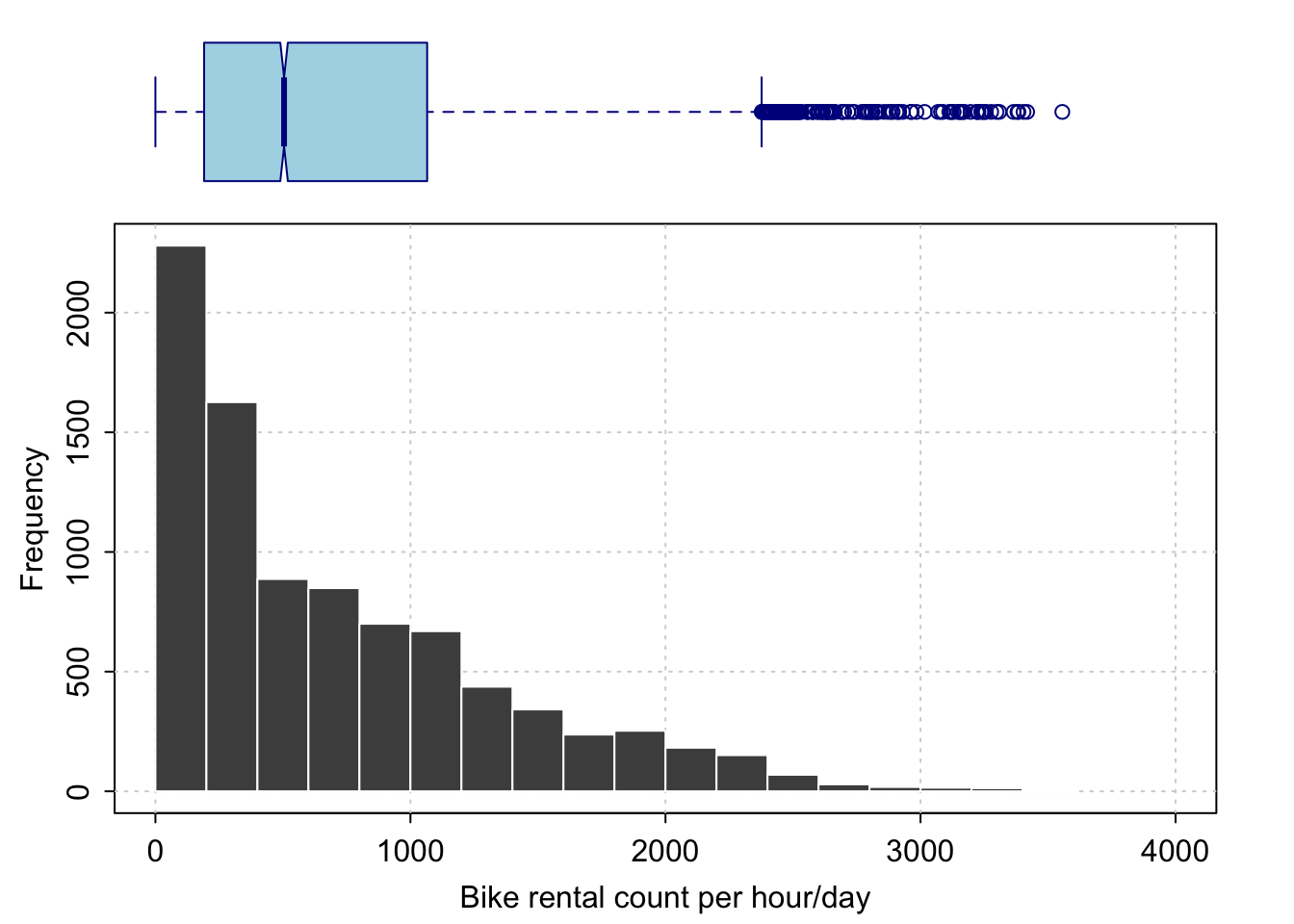
There is one data point that might be considered as an ourlier, as it is several hundred counts above the rest.
Here is a summary of that point. Given that it occured at 6pm in what might be ideal cycling weather (24C temp, low humidity), I would suggest this is a true high rather than a false measurement.
bike[bike$Rental.Count > 3500,]1.4 Univariate Modelling
(In future weeks we might skip this)
1.4.1 Model 1: Normal Distribution
1.4.1.1 Model description:
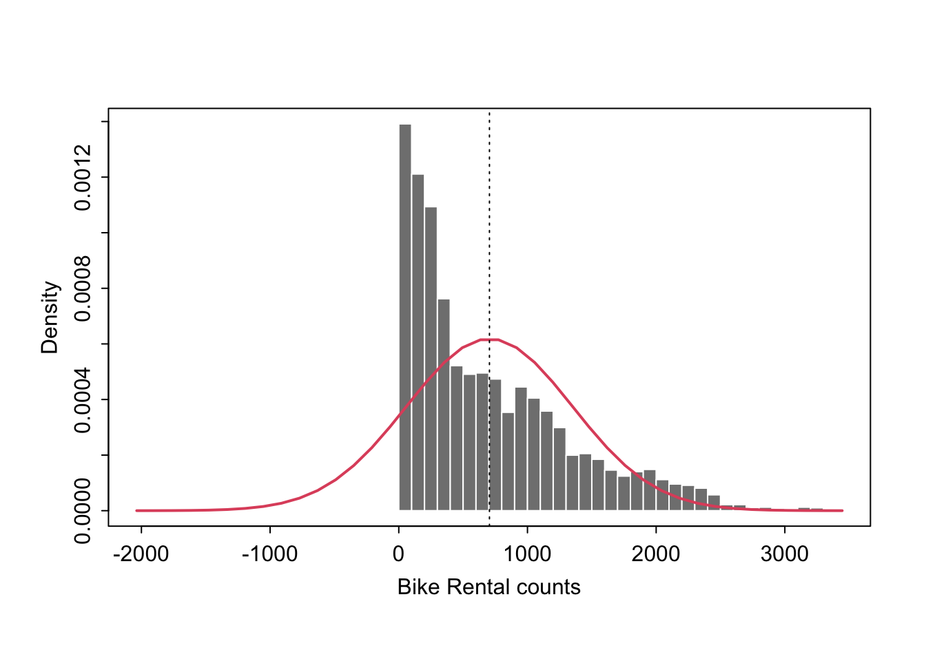
As my first model, I suggest that we don’t know a predictor that can explain bike rental count. Instead, I am going with the most basic model possible, that we can model rental count for the population as a Normal Distribution \(~N(\mu_y, {\sigma_y}^2)\) with true mean equal to my sample mean: \(~N(\mu_y, {\sigma_y}^2)\) with \(\mu_y=\bar{y}=704.6\) counts per hour.
For example:
1.4.1.2 Model validity:
From my exploratory histogram and the plot above, I can see some clear issues with this model. The first is our problem of count data! We cannot have negative counts, yet our model will clearly predict negatives.
Secondly the model looks highly skewed. We can further assess this using a QQ-Plot and a Wilk-Shapiro hypothesis test:
ggqqplot(bike$Rental.Count,col="red")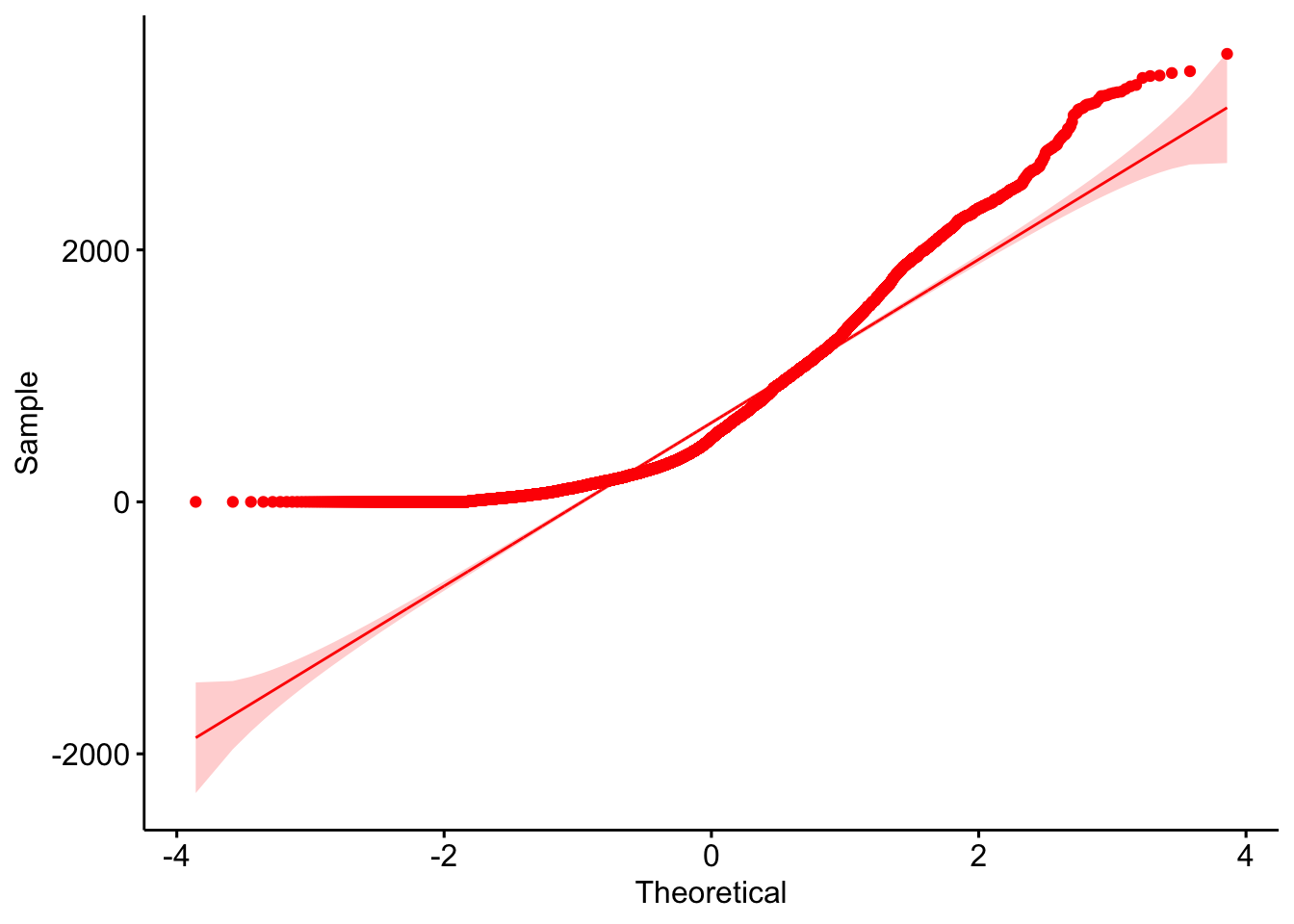
We know that Wilk-Shapiro is very sensitive to normality for large datasets, so we already know the answer here, but as proof:
# My original dataset was too big for the command, so I sampled 3000 random values
shapiro.test(sample(bike$Rental.Count,3000))
##
## Shapiro-Wilk normality test
##
## data: sample(bike$Rental.Count, 3000)
## W = 0.87962, p-value < 2.2e-16H0: Our dataset was sampled from an underlying normal distribution, \(~N(\mu_y, {\sigma_y}^2)\) with \(\mu_y=\bar{y}=704.6\) and \({\sigma_y}^2={s_y}^2=416021\) counts per hour.
H1: The Wilks-Shapiro test statistic is unusually low compared to expected from the Normally Distributed population described in H0.
Our test statistic above is 0.885 with a p-value of effectively zero. It would be incredibly unlikely for this result to have occurred by chance if the data really was normal.
The result of this test means that our model is likely to be useful in understanding population parameters such as the population mean, but it will NOT be useful in predicting new values.
1.4.1.3 Assessing population parameters:
As described above, the Central Limit Theorem means that this model even though flawed, will still be useful in predicting the population mean, using the equation:
\[ \bar{y} ± T_{(n-1),(1-\frac{\alpha}{2})}\frac{s_y}{\sqrt{n}} \]
where we use a T distribution with n-1 degrees of freedom (n is the number in the sample) and alpha is the confidence level. As the sample size is so big, this is functionally a Normal distribution.
Here I calculate the 99th percentile confidence interval on the population mean:
mytest <- t.test(bike$Rental.Count, conf.level = .99)

conf.lower <- mytest$conf.int[1]
conf.upper <- mytest$conf.int[1]

mytest
##
## One Sample t-test
##
## data: bike$Rental.Count
## t = 102.24, df = 8759, p-value < 2.2e-16
## alternative hypothesis: true mean is not equal to 0
## 99 percent confidence interval:
## 686.8472 722.3569
## sample estimates:
## mean of x
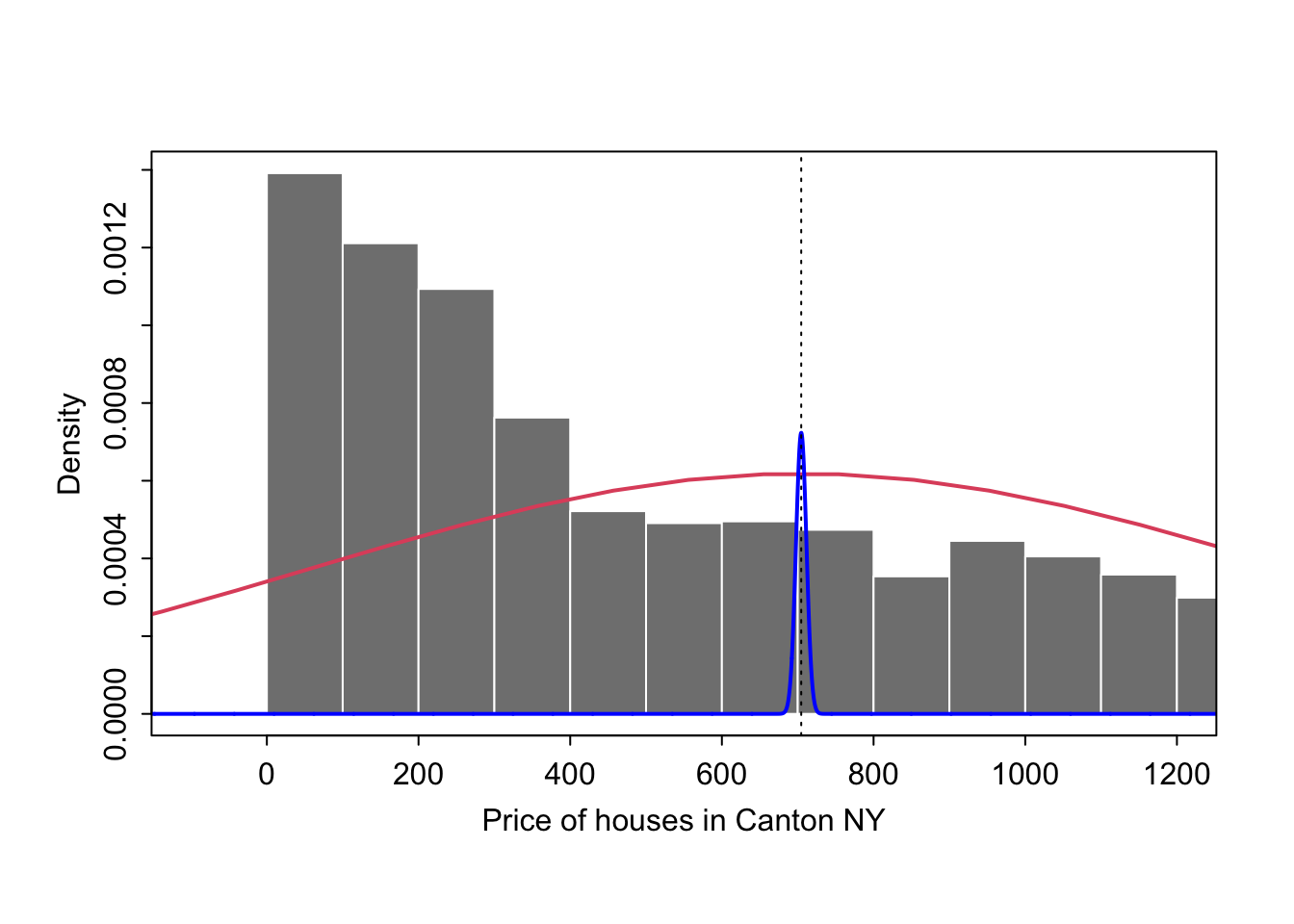
## 704.6021This means that given our sample, we are 99% sure that the true population mean falls in the range 686.8471771 to 686.8471771 rentals per hour. We are essentually saying that the true mean falls inside the blue curve, which has mean \(~N(\mu_y, {\sigma_y}^2)\) and standard deviation: \(\frac{{s_y}}{\sqrt{n}}\)
1.4.1.4 Testing the population mean
My client has requested I assess the likelihood that the true mean rental is ABOVE 700 counts per day. I can do this using a one sided T-test on the population mean with test statistic:
\[ T=\frac{\bar{y}-\mu_y}{\frac{s_y}{\sqrt{n}}} \]
H0: Our dataset was sampled from an underlying normal distribution with true mean, \(\mu_y = 700\)
H1: The observed test statistic is unusually high if H_0_ was true, therefore we think, \(\mu_y > 700\)
The critical significance is 80%. By this I think my client meant to say that they want to be 80% certain, so I am taking my critical p value as 0.2.
The T-test above tests the likelyhood that the true mean was zero! But it is easy to adapt.
mytest <- t.test(bike$Rental.Count, mu=700, alternative="greater")
mytest
##
## One Sample t-test
##
## data: bike$Rental.Count
## t = 0.6678, df = 8759, p-value = 0.2521
## alternative hypothesis: true mean is greater than 700
## 95 percent confidence interval:
## 693.2656 Inf
## sample estimates:
## mean of x
## 704.6021knitr::include_graphics("./Figures/tttest_plot.png")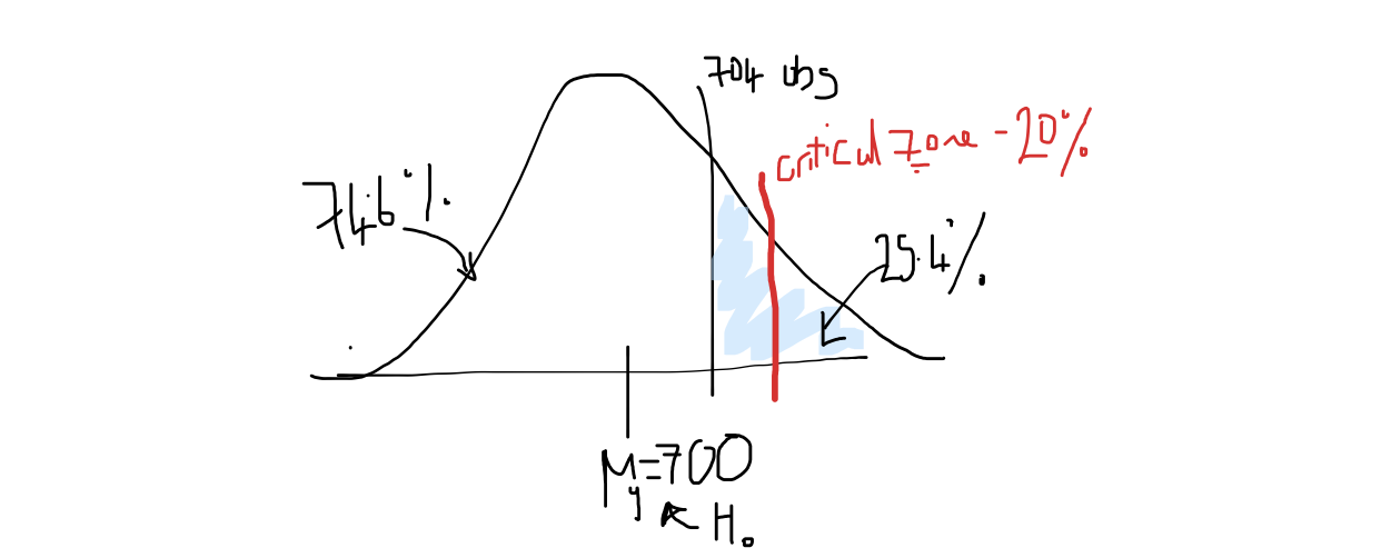
So in this case, we can see that the observed result is not extreme enough to be only observed 20% of the time. As p=0.254 > 0.2, there is not enough evidence to reject the null hypothesis.
Given our sample, there is nothing to suggest the true mean is greater than 700 rentals per day.
1.4.1.5 Model predictions
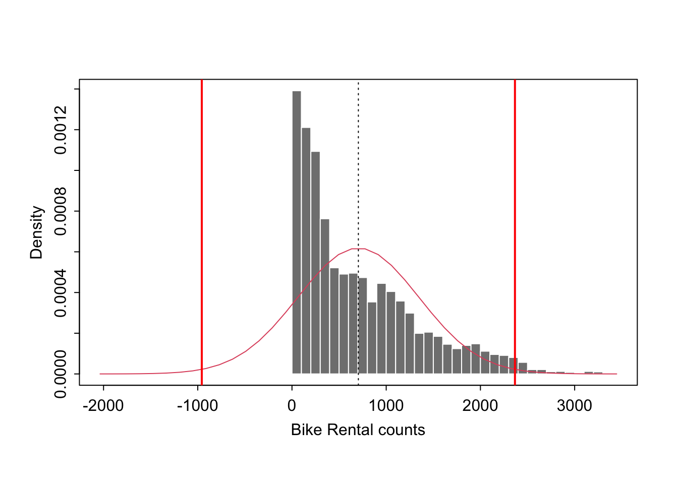
Given the fact our data is clearly not normal (see model validity), this is clearly not appropriate. But at my clients request, here is a 99% prediction interval for our data.
\[ \bar{y} ± T_{(n-1),(1-\frac{\alpha}{2})} s_y \sqrt{1+\frac{1}{n}} \]
n <- nrow(bike)
df=n-1
ybar <- mean(bike$Rental.Count)
sy <- sd(bike$Rental.Count)

lowerPI.99 <- mean(bike$Rental.Count) - qt(0.995,df) * sy * (sqrt(1+(1/n)))
upperPI.99 <- mean(bike$Rental.Count) + qt(0.995,df) * sy * (sqrt(1+(1/n)))

lowerPI.99
## [1] -957.2583upperPI.99## [1] 2366.462If our model is true (it’s clearly not), we suggest that we are 99% sure that a new hourly record of bike rental will fall between -957 and 2366.
So for example, according to this Normal univariate model, we are 99% sure that we won’t see a new rental day of hour with over 3000 rentals. This is clearly nonsense!
1.5 Bivariate models
1.5.1 Exploratory analysis of predictors
I suspect that temperature might impact my bike rental counts, and wish to assess this and other predictors. To do this, I can first assess the correlation of all the predictors together
First, to summarise the correlation between our numeric variables:
library(corrplot)
bike.numeric.columns <- bike[ , sapply(bike,is.numeric)]

corrplot(cor(bike.numeric.columns),method="ellipse",type="lower")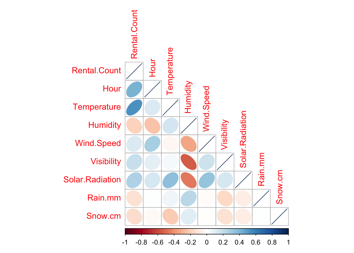
We can see that there is a relatively strong link with temperature. Looking in more detail below, the correlation between bike rental count and temperature is 0.539.
library(GGally)
ggpairs(bike[,c("Rental.Count","Hour" ,"Temperature","Humidity" , "Season"   )],cex=.3)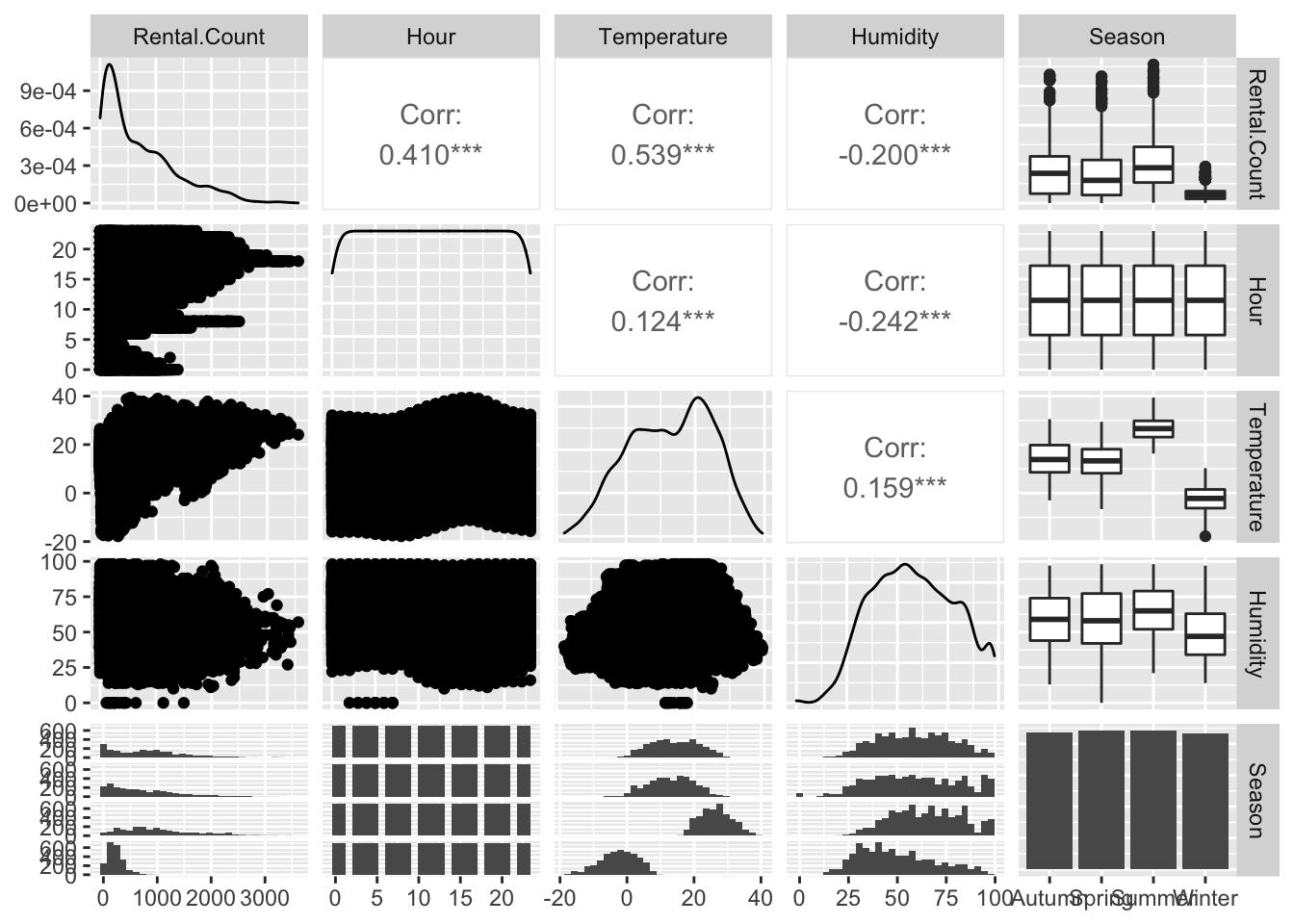
ggpairs(bike[,c("Rental.Count","Wind.Speed" ,"Visibility","Solar.Radiation" , "Snow.cm" ,"Holiday" )])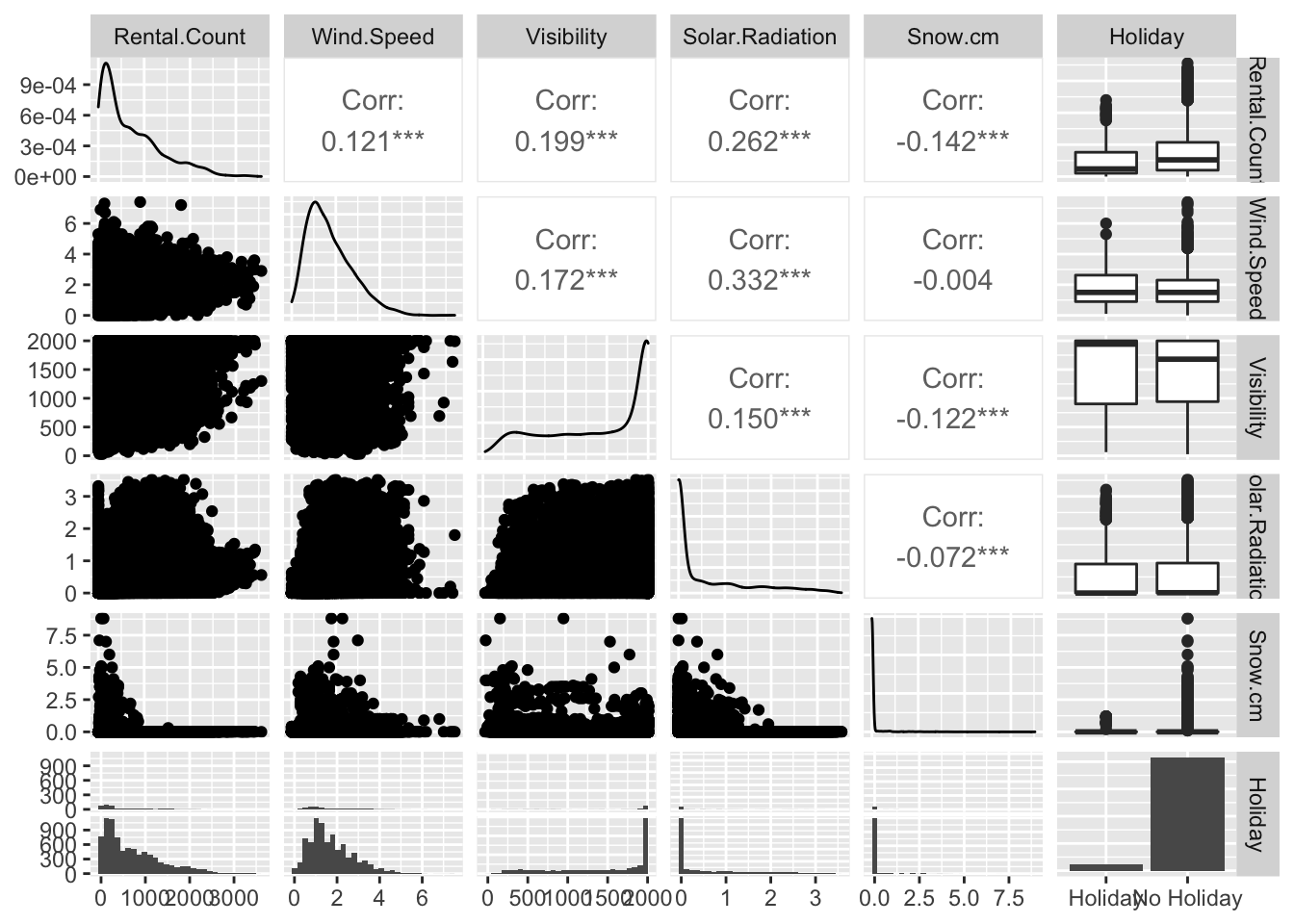
1.5.2 Model 2: Temperature predicts rental count
- response variable, rental count per hour
- predictor, temperature (C)
- unit of analysis (an hour)
# Basic scatter plot.
ggplot(bike, aes(x=Temperature, y=Rental.Count)) +
geom_point( color="dark red",size=.3) 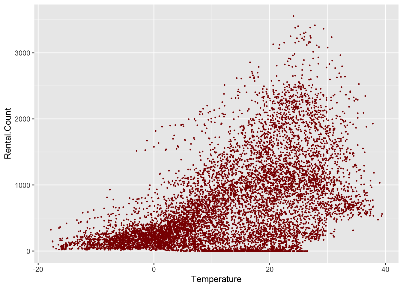
Here we see a moderately strong positive relationship between temperature and rental count. There does appear to be some complex clustering within the data however and although potentially the average rental count increases linearly, there is meaningful heteroskadisity (the variance increases with temperature).
1.5.2.1 Model description
My new model is that the population rental count can be modelled as a Normal Distribution \(~N(\mu_y, {\sigma_y}^2)\) , but where the true mean, _y increases linearly with temperature, Temp. e.g.
\[ \mu_y = \beta_0+\beta_1Temp \]
Using least squares to fit this model we find:
model2 <- lm(Rental.Count ~ Temperature, data=bike)
model2
##
## Call:
## lm(formula = Rental.Count ~ Temperature, data = bike)
##
## Coefficients:
## (Intercept) Temperature
## 329.95 29.08equatiomatic::extract_eq(model2,use_coefs = TRUE)\[ \operatorname{\widehat{Rental.Count}} = 329.95 + 29.08(\operatorname{Temperature}) \]
and with summary statistics
olsrr::ols_regress(model2)## Model Summary
## ------------------------------------------------------------------
## R 0.539 RMSE 543.498
## R-Squared 0.290 Coef. Var 77.136
## Adj. R-Squared 0.290 MSE 295390.482
## Pred R-Squared 0.290 MAE 403.832
## ------------------------------------------------------------------
## RMSE: Root Mean Square Error
## MSE: Mean Square Error
## MAE: Mean Absolute Error
##
## ANOVA
## ---------------------------------------------------------------------------------
## Sum of
## Squares DF Mean Square F Sig.
## ---------------------------------------------------------------------------------
## Regression 1056904520.199 1 1056904520.199 3577.991 0.0000
## Residual 2587029842.564 8758 295390.482
## Total 3643934362.763 8759
## ---------------------------------------------------------------------------------
##
## Parameter Estimates
## -------------------------------------------------------------------------------------------
## model Beta Std. Error Std. Beta t Sig lower upper
## -------------------------------------------------------------------------------------------
## (Intercept) 329.953 8.541 38.631 0.000 313.210 346.695
## Temperature 29.081 0.486 0.539 59.816 0.000 28.128 30.034
## -------------------------------------------------------------------------------------------This can be plotted as follows:
library(hrbrthemes)

# Basic scatter plot.
ggplot(bike, aes(x=Temperature, y=Rental.Count)) +
  geom_point(size=.5) +
  geom_smooth(method=lm , color="red", se=FALSE)  +
  theme_ipsum()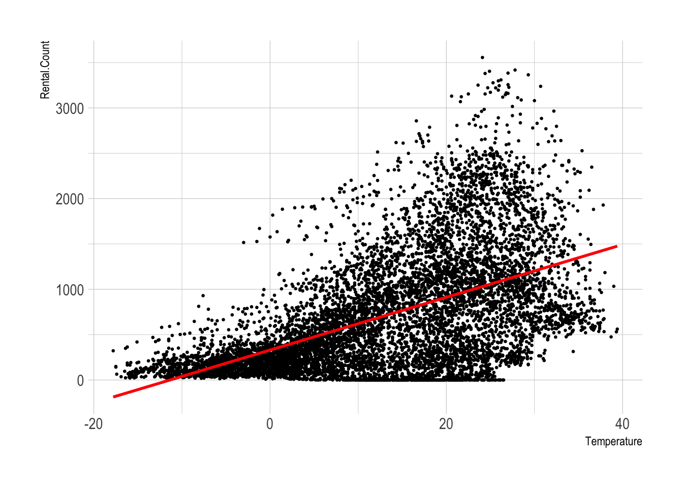
1.5.3 Model validity
1.5.3.1 Independence & confounding variables
I do have concerns about independence, especially that hour of day might impact rental count:
# create the plot, save it as "p" rather than print immediatly
myplot <-   ggplot(bike, aes(x=Temperature, y=Rental.Count,color=Hour)) +
            geom_point(alpha=.5) +
            theme_classic()+
            scale_color_gradient(low="blue", high="red")

# and plot interactively
ggplotly(myplot)
This makes physical sense. People are less likely to rent bikes late at night when it is also likely to be colder. So it might be that my model needs to improve, with hour also added to the model.
1.6 Conclusions
So far, I have shown that the average rental count per hour is approximately 700 counts/hr, with a highly skewed histogram ranging from 0 to around 3000. Temperature appears to impact the average rental count.