Chapter 2 Lab 1

Welcome to STAT-462 labs. The aim of this week is to:

Become familiar with the RStudio and RMarkdown interface
Learn about projects and libraries
Start using R commands (known as functions)
Understand R Markdown and the process for submitting assignments
Do some basic data analysis

If the labs are causing major problems with your computer or your computer hardware is struggling (or you have any other software issue), Talk to Dr Greatrex. We can fix this and there are other options for “online R” that you can use. As these all have their own issues, getting it installed on your computer is likely easiest and the one I would like you to try first.

In general, you can reach out to any of the teaching staff if you have any issue at all - we have likely see the errors hundreds of times before and we are happy to help. There is also a canvas discussion board for this lab which will be the fastest place to get an answer. https://psu.instructure.com/courses/2115020/discussion_topics/13706473

2.1 Getting started

2.1.1 Why is this class in R?

There are many different types of software one can use to analyze spatial data. We’re going to focus on the R programming language because:

It’s free and open source.
It allows you to do traditional statistics, machine learning and data analysis.
It’s a good introduction to programming, which is great for your resume.
There are some great visualization tools you can use to allow R to make your own professional books, websites, resumes, presentations and interactive tools. We will explore many of these in the class

2.1.2 Installing R and R-studio

In this class, we would like you to download and install BOTH R and R-Studio onto your own computers. You should have already completed this step for Homework 1. If you have not, see instructions here: https://psu.instructure.com/courses/2115020/assignments/12682456

FOR WINDOWS USERS. Sometimes R asks you to download something called RTools. You can do so here: https://cran.r-project.org/bin/windows/Rtools/ Follow the instructions closely and ask if you need support.

2.1.3 Open R-studio

Figure 2.1: Icons of the R program and R-studio

Open R-studio (NOT R!). You should be greeted by three panels:

The interactive R console (entire left)
Environment/History (tabbed in upper right)
Files/Plots/Packages/Help/Viewer (tabbed in lower right)

If you click on the View/Panes/Pane Layout menu item, you can move these quadrants around. I tend to like the console to be top left and scripts to be top right, with the plots and environment on the bottom - but this is totally personal choice.

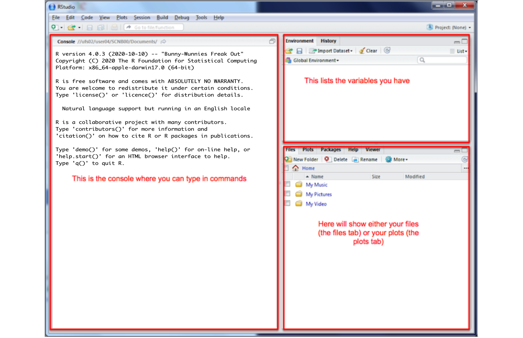
Figure 2.2: The basic R-studio screen when you log on

If you wish to learn more about what these windows do, have a look at this resource, from the Pirates Guide to R: https://bookdown.org/ndphillips/YaRrr/the-four-rstudio-windows.html

If you have used R before, you might see that there are variables and plots etc already loaded. It is always good to clear these before you start a new analysis. To do this, click the little broom symbol in your environment tab.

2.1.4 Change a few settings

R-studio wants to be helpful and will try to re-load exactly where you were in a project when you log back in. This can get really confusing, so we are going to turn this off.

ON A MAC: Click on the R-studio menu button on the top left of the screen, then click Preferences.

ON A PC: Click on Tools-> Global Options -> Preferences

Now:

UNCLICK “Restore most recently opened project at startup”
Set “Save workspace to .RData on” exit to Never

2.2 Lab challenge 1

2.2.1 What are projects?

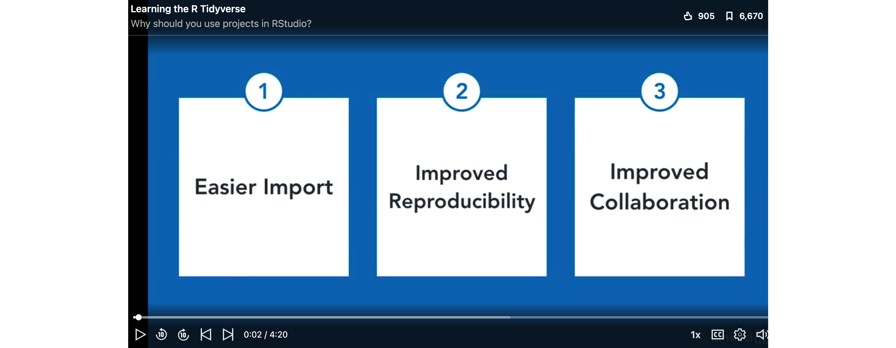
One of the most useful new features in RStudio are R-Projects. We are going to use R-projects to store our lab data in. An R project is a place to store all your commands, data and output in the same place.

Before R projects, we had to worry about where on your computer your data was saved in. Now, we can force R-Studio to immediately look inside your lab folder - making life much easier.

Equally, projects allow you to have multiple versions of R-studio open. This is useful because say you have Lab-2 open, but want to re-open Lab-1 to check some code, clicking the “Lab 1 project file” will load a whole new version of R with Lab 1 ready to edit.

It is really important that you stay organized in this course, for example making sure you know where you put your data and your labs.

To encourage this, choose a place that makes sense on your computer, create a folder called STAT-462. can either do this outside R studio in your file explorer, or inside the “Files tab” in R studio. You should store all your 462 labs inside this folder

Now we will create our first project (also see the pic):

open R-Studio and click New Project,
then click “new directory”
then “new project”.
Name your project Lab 1, then browse to your newly created STAT-462 folder and press open.
Press OK and your project is created.
- You will also see that a new sub-folder has been created in your STAT-462 folder called Lab 1
- Inside that is your Project file. (with a .Rproj extension)

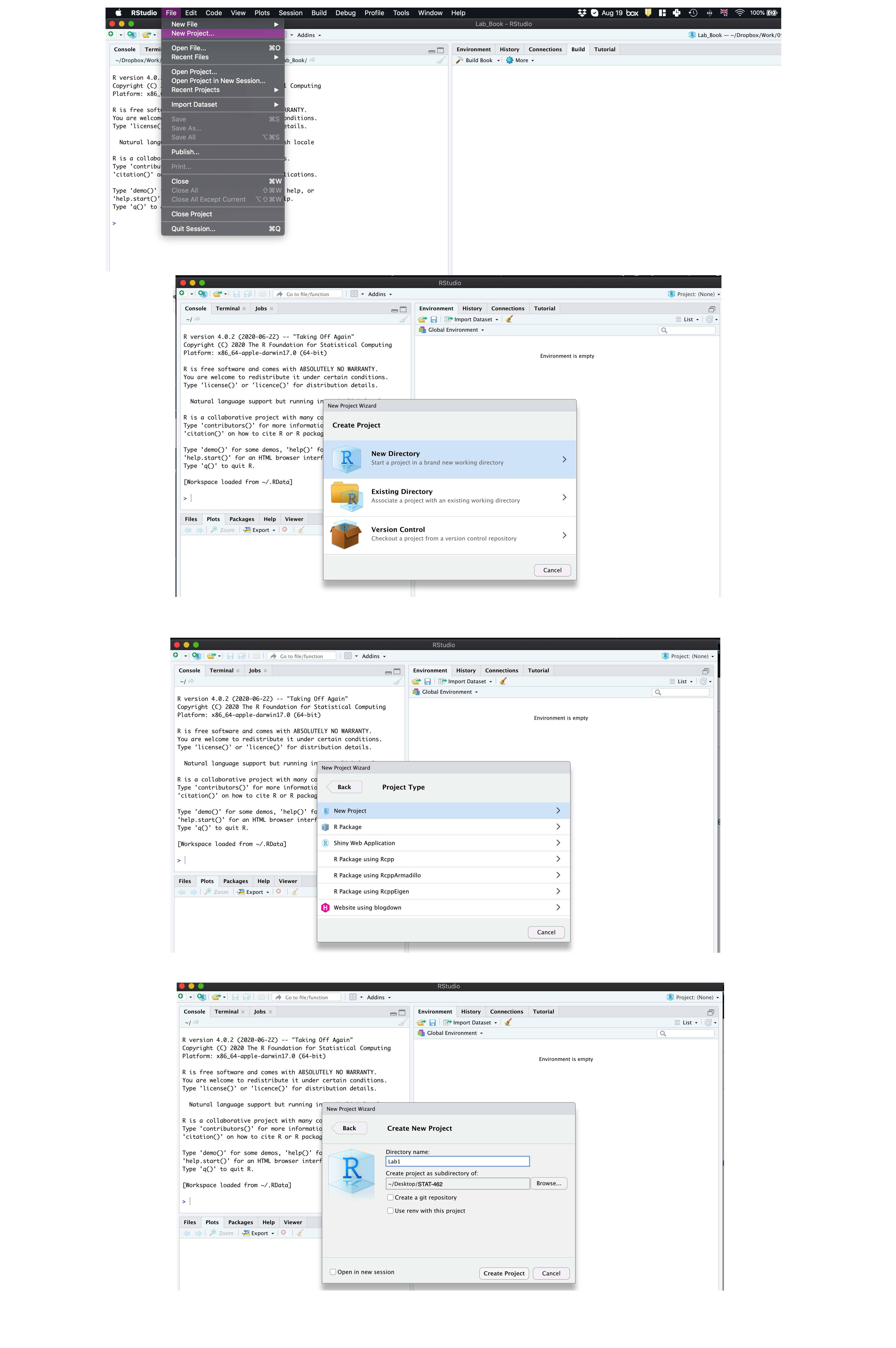
Figure 2.3: Instructions to create an R project

Your output should look something like this:

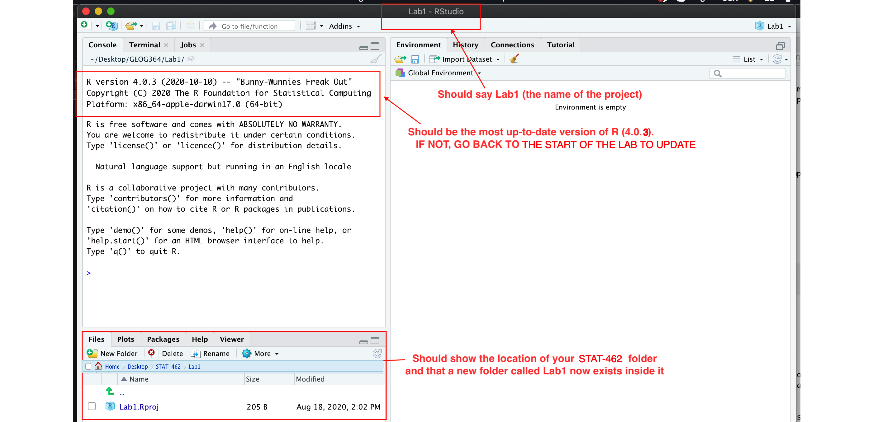
Figure 2.4: What you should see

Equally, R should now be “looking” inside your Lab 1 folder, making it easier to find your data and output your results. Try typing this into the console (INCLUDING THE EMPTY PARANTHESES/BRACKETS) and see if it prints out the location of Lab 1 on your computer. If not, talk to an instructor.

getwd()

In the future, every time you want to work on Lab 1, rather than open R-studio directly, double click the R project file inside Lab 1 and you will get back to your work.

If you’re having issues at this point or haven’t managed to get to this step, STOP! Ask an instructor for help.

Now you have opened your project, take a screenshot of your R-studio page. It should look like Figure 2.4, e.g. with at least R version 4.0.3, with the Lab 1 project and the project stored in your STAT-462 folder.

To take a screenshot on a mac, press Command-3. The screenshot will appear on your desktop
To take a screenshot on a PC, press Alt + PrtScn

Rename the screenshot to your “username_Lab1_Fig1”(for example for me it will be hlg5155_Lab1_Fig1), then place it in your Lab 1 sub-folder inside STAT-462. This folder was created when you made the project.

You will need this later, so don’t skip this step.

2.3 R coding basics

So now we FINALLY get to do some R-coding. First things first, first watch the 5 min video above for some pointers. Will will also go through this below:

2.3.0.1 Using R as a calculator

Remember that the aim of R is to type in commands to get your computer to analyse data. The console (see Figure 2.2) is a space where you can type in those commands and it will directly print out the answer. You’re essentially talking to the computer.

The little “>” symbol in the console means that the computer is waiting for your command.

Let’s start by the simplest command possible. Try typing each of the following commands into your R console and pressing Enter as you work through this.

1+1

## [1] 2

Note that spacing does not matter: 1+1 will generate the same answer as 1 + 1.

When using R as a calculator, the order of operations is the same as you would have learned back in school, so use brackets to force a different order. For example,

3 + 5 * 2

## [1] 13

will give a different result to

(3 + 5) * 2

## [1] 16

2.3.0.2 Adding text

Now for text. Can you say hello world?

Figure 2.5: Your screen after running the project

Nope, there is an error! To make R understand text, it is important to use quote marks.

print("Hello World")

## [1] "Hello World"

2.3.0.3 Comparisons

We can also do comparisons in R - using the special symbols TRUE or FALSE (no quote marks, they are special).

Here we are asking R whether 1 is equal to 1.

# note two equals signs is read as "is equal to"
1 == 1

## [1] TRUE

We could also have used

!= “Not equal to”
< “Less than”
<= "Less than or equal to`
> “Greater than”
>= “Greater than or equal to”

What if I press Enter too soon?

If you type in an incomplete command, R will wait for you to complete it. For example, if you type 1 + and press enter, R will know that you need to complete the command So it will move onto the next line but the > will have changed into a +, which means its waiting for you to complete the command.

If you want to cancel a command you can simply hit the “Esc” key or press the little stop symbol and R studio will reset.

Pressing escape isn’t only useful for killing incomplete commands: you can also use it to tell R to stop running code (for example if it’s taking much longer than you expect), or to get rid of the code you’re currently writing.

2.3.1 Variables and assignment

It’s great to be able to do maths easily on the screen, but really we want to be able to save our results, or load in data so we can run more complex commands. In R, we can give our data a name e.g. we save our data as a variable. So then, instead of typing the whole command, we can simply type the variable’s name and R will recall the answer.

The symbol to store data into a variable is using the assignment arrow <-, which is made up of the left arrow and a dash. You can also use the equals sign, but it can cause complications later on. Try typing this command into the console:

x <- 1/50

Notice that pressing enter did not print a value onto your screen as it did earlier. Instead, we stored it for later in something called a variable, with the name ‘x’.

So our variable x is now associated with the value 0.02, or 1/50. You can print a variable on screen by typing its name, no quotes, or by using the print command. Try printing out your variable.

## [1] 0.02

# or

print(x)

## [1] 0.02

Look for the Environment tab in one of the panes of RStudio, and you will see that ‘x’ and its value have appeared. This ‘x’ variable can be used in place of a number in any calculation that expects a number. Try typing

log(x)

## [1] -3.912023

Notice also that variables can be reassigned:

x <- 100
print(x)

## [1] 100

x used to contain the value 0.025 and and now it has the value 100.

Note, the letter x isn’t special in any way, it’s just a variable name. You can replace it with any word you like as long as it contains no spaces and doesn’t begin with a number. Different people use different conventions for long variable names, these include

periods.between.words.1
underscores_between_words
camelCaseToSeparateWords

What you use is up to you, but be consistent.

Finally, R IS CASE SENSITIVE. X and x are different variables!

h <- 1
H <- 2

ans <- h+H
print(ans)

## [1] 3

Combining variables

As I showed above, you can now use multiple variables together in more complex commands. For example, try these commands:

#Take the variable x, add 1 then save it to a new variable called y
y <- x + 1 
# print the multiple of 2yx onto the screen
y

## [1] 101

Now you can see that there are two variables in your environment tab, x and y. Where y is the sum of the contents of x plus 1.

The way R works is that first it looks for the commands on the right of the arrow. It runs all of them, calculates the result, then saves that result with the name on the left of the arrow. It does not save the command itself, just the answer. For example, in this case, R has no idea that y was created using a sum, it just knows that it is equal to the number 3.

You can even use this to change your original variable . Try typing the code below in a few times into the console and see what happens.

A short cut to do this is to type the commands the first time, then use the up-arrow on your keyboard to cycle back through previous commands you have typed

x <- x + 1 # notice how RStudio updates its description of x in the environment tab
x          # print the contents of "x" onto the screen

## [1] 101

Our variables don’t have to be numbers. They could refer to tables of data, or a spatial map, or any other complex thing. We will cover this more in future labs.

2.3.2 Functions

A command is simply an action you can take - like pressing the square root button on a calculator, followed by the number you wish to take the square root of. A command is always followed by parentheses ( ), inside which you put your arguments.

The power of R lies in its many thousands of these built in commands, or functions. In fact, we have already come across one - the print command. Some more examples include:

plot(x=1:10,y=1:10)
- This will plot the numbers 1 to 10 against 1 to 10
x <- nchar("hello")
- This will count the number of letters in the word “hello” (e.g. 5), then save it as a variable called x

Watch this short video to learn three important facts about functions:

One example of a function is file.choose() (not how I put the parentheses in this lab book so you can see it is a command). This command will let you interactively select a file and print the address out onto the screen.

Try each of these out in your console for the file.choose() command, leaving the parentheses blank.

# Typing this into the console will print out the underlying code
file.choose 

# Typing it WITH parentheses will run the command.  
file.choose()

# Typing a ? in front will open the help file for that command
?file.choose

Sometimes we need to give the command some additional information. Anything we wish to tell the command should be included inside the inside the parentheses (separated by commas). The command will literally only know about the stuff inside the parentheses.

sin(1) # trigonometry functions.  Apply the sine function to the number 1.

## [1] 0.841471

log(10) # natural logarithm.  Take the natural logarithm of the number 10.

## [1] 2.302585

This following command will plot the number 1 to 10 against the numbers 12 to 20, along with some axis labels. When you run this, the plot will show up in the plots tab.

# plot the numbers 1 to 10 against the numbers 11 to 20
plot(1:10,11:20,col="dark blue", xlab="x values",ylab="STAT-462 is the best")

If you are feeling lost, https://swcarpentry.github.io/r-novice-gapminder/01-rstudio-intro/ is a really good website which goes over a lot of this in more detail. A lot of this is based on their work.

2.3.3 Packages

There are now several million commands/functions available for you to use in R. To make sure your computer doesn’t get overwhelmed, it doesn’t load all of these at once. In fact many need to be downloaded from the internet.

So we have

R: The programming language itself
Functions: Specific commands or actions written in the R language
Packages: Commands are grouped into bundles/apps called packages, which we download from the internet and load every time we need them.

A close analogy is your phone. There are millions of apps available from banking, to social media to camera filters. You don’t have every app in the world installed on your phone - and you don’t have every app you do download running at the same time.

This is the same for R:

You download and install packages from the internet that you might need. This can be done by clicking the install button in the Packages tab. Or you can use the install.packages() command. You only ever need to do this once.
To actually run the commands in the package you need to load/run them - just in the way you tap an app to start it. This can be done using the library() command.

2.4 Lab Challenge 2

Now we are going to download some packages from the internet and install them. You must be connected to the internet to make this happen! In the console, type the following commands, or click the “Install” button in the packages tab (next to plots) and find the package name. If it asks if you want to install dependencies, say yes.

If R gives you warnings about rtools, ignore them or follow the instructions at the top to install R-Tools.

# COPY/PASTE THESE INTO YOUR CONSOLE AND LET THEM RUN. 
#(These are hopefully all the packages for the course, so it's a one off download)

install.packages("tidyverse") # Lots of data processing commands
install.packages("knitr")     # Helps make good output files
install.packages("rmarkdown") # Helps make good output files
install.packages("lattice")   # Makes nice plots
install.packages("RColorBrewer") # Makes nice color-scales
install.packages("ISLR")      # contains a credit dataset
install.packages("yarrr")     # contains a toy dataset about pirates
install.packages("skimr")     # Summary statistics
install.packages("Stat2Data") # Regression specific commands
install.packages("olsrr")     # Regression specific commands
install.packages("nortest")   # Regression specific commands
install.packages("lmtest")    # Regression specific commands
install.packages("IMTest")    # Regression specific commands 
install.packages("MASS")      # Regression specific commands
install.packages("moderndive")# Regression specific commands
install.packages("corrplot")  # correlation plots
install.packages("ggpubr")    # Nice regression plots
install.packages("car")       # this one sometimes has problems, don't panic if you get errors

You will see a load of red text appear in the console as it tells you its very detailed status of how it’s downloading and installing. Don’t panic! It might also take several minutes to do this, longer on a bad internet connection. We are doing this as a one off at the start of the course.

When you have run all the commands and waited until they have finished running (remember, when it is done, you should see the little “>” symbol in the console waiting for your next command), we want to check if they have installed successfully onto your computer.

To do this we are going to load them using the library command:

library("tidyverse") # Lots of data processing commands
library("knitr")     # Helps make good output files
library("rmarkdown") # Helps make good output files
library("lattice")   # Makes nice plots
library("RColorBrewer") # Makes nice color-scales
library("ISLR")      # contains a credit dataset
library("yarrr")     # contains a toy dataset about pirates
library("skimr")     # Summary statistics
library("Stat2Data") # Regression specific commands
library("olsrr")     # Regression specific commands
library("nortest")   # Regression specific commands
library("lmtest")    # Regression specific commands
library("IMTest")    # Regression specific commands 
library("MASS")      # Regression specific commands
library("moderndive")# Regression specific commands
library("corrplot")  # correlation plots
library("ggpubr")    # Nice regression plots
library("car")       # this one sometimes has problems, don't panic if you get errors

If you have managed to install them successfully, often nothing happens - this is great! It means it loaded the package without errors.

Sometimes, it will tell you friendly messages. For example, this is what shows up when you install the tidyverse package. It is telling you the sub-packages that it downloaded and also that some commands, like filter - now have a different meaning. E.g. originally the filter command did one thing, but now the tidyverse package has made filter do something else.

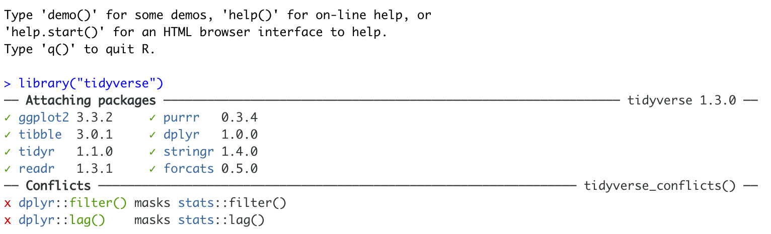
Figure 2.6: Tidyverse install messages

To find out if what you are seeing is a friendly message or an error, run the command again. If you run it a second time and there is no error then nothing should happen.

! IMPORTANT If you see some red errors here after multiple attempts running the commands, we will have to fix what your computer is doing together. If you see errors, then take a screenshot of the full page and talk to a TA or Dr Greatrex, or post on the Lab 1 discussion.

Note - you don’t need to submit anything for lab challenge 2 - it’s here to make the rest of the semester run smoothly. Your only action is to reach out if there are errors.

2.5 Markdown & Exploratory Analysis

2.5.1 What is R-markdown?

So far, we’ve been typing commands into the console, but these will all be lost once you close R. Equally, it’s hard to remember or reproduce the analysis you have done . So we will now move onto writing code commands that you can save and submit.

There are several types of document that you can create and save in R-Studio.

A basic script (the filetype is .r). This is simply just a blank document where you can save code commands. When you “run” the commands in the script, R simply copy/pastes the commands over to the console.
An R-Notebook or R-Markdown document (the filetype is .Rmd). These are documents you can use to write a report with normal text/pictures, but and also include both your R code and output. You can turn these into reports, websites, blogs, presentations or applications. For example these instructions are created using a markdown document.

In this course we are going to focus on the R-Markdown format and you are going to submit your labs as html files.

2.5.2 Creating a markdown document

Time to make your own. Go to the File menu on the top left, then click New File - R-Markdown. It will ask you to name and save your file. Call it STAT-462 Lab 1.

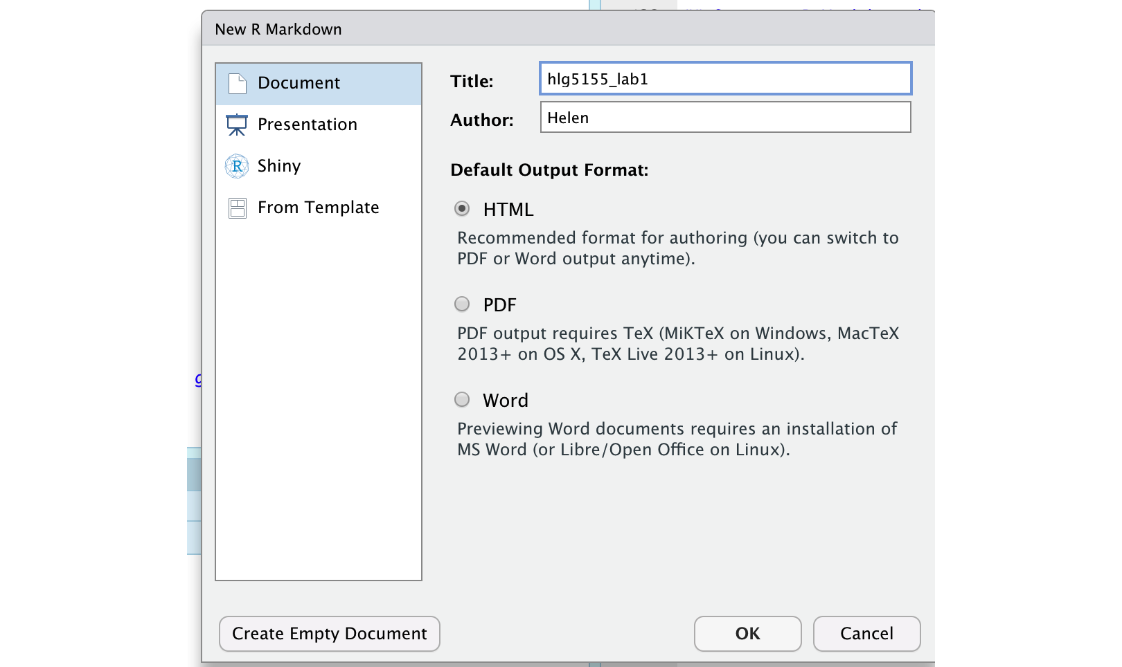
Figure 2.7: You should see TWO new files appear in your lab 1 folder

A file should appear on your screen - your first markdown script. Essentially, we have some space for text, some space for code, and a space at the top of the file where we can add information about themes/styles etc. Each file contains some friendly text to explain what is going on, which I have annotated here.

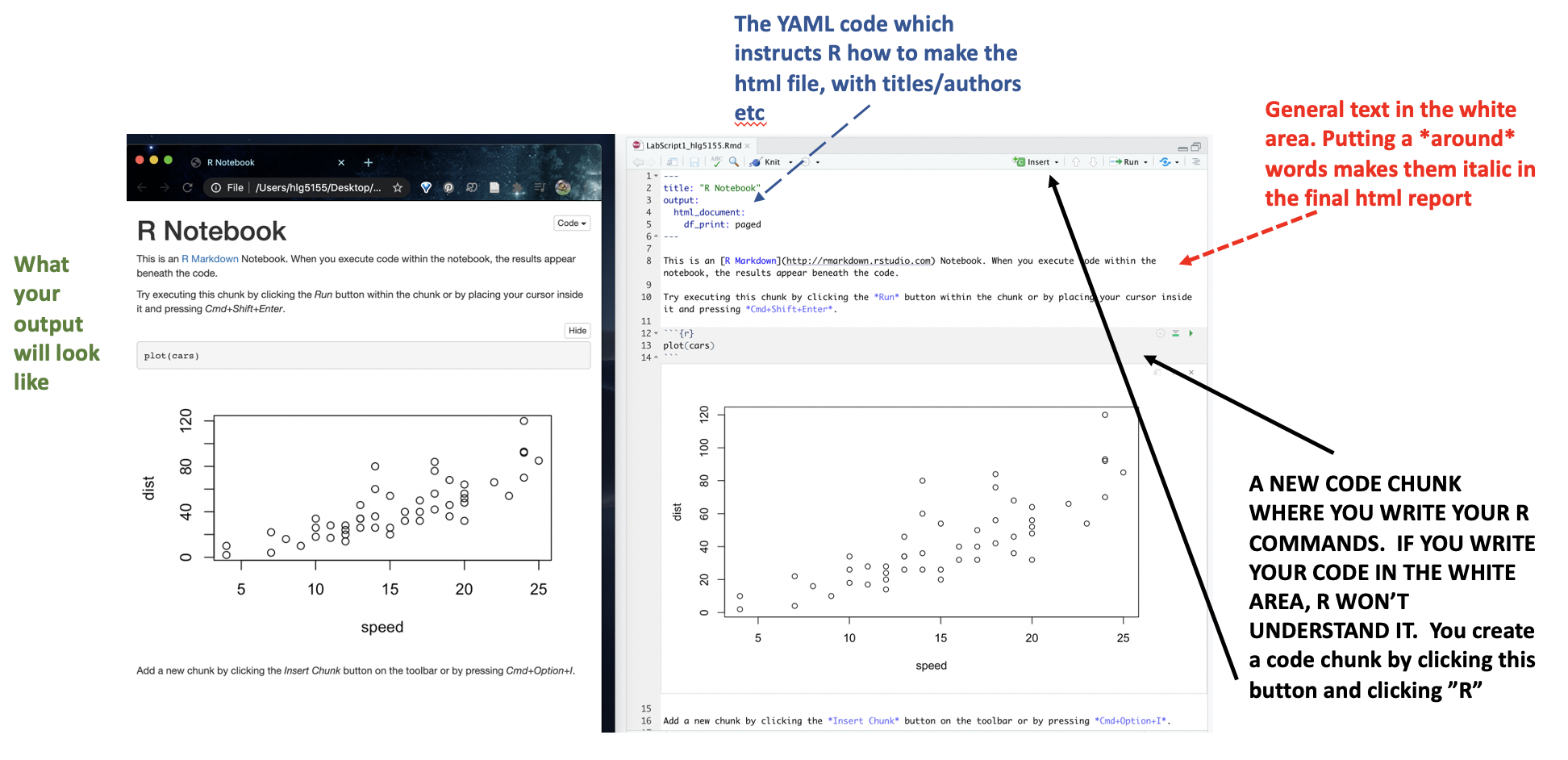
Figure 2.8: You should see TWO new files appear in your lab 1 folder

Code chunks are the grey areas and are essentially “mini consoles”. If you click on the little right triangle arrow at the top-right of the code chunk, you can run the plot command, and a plot will appear, running the code.

Note, it no longer runs in the console. You can still copy things into the console, by clicking on the line you want to run and pressing Ctrl-Enter / command-Enter.

Let’s try this. On line 11, delete plot(cars) and type 1+1. Now press the green arrow and the answer should appear directly under your code chunk.

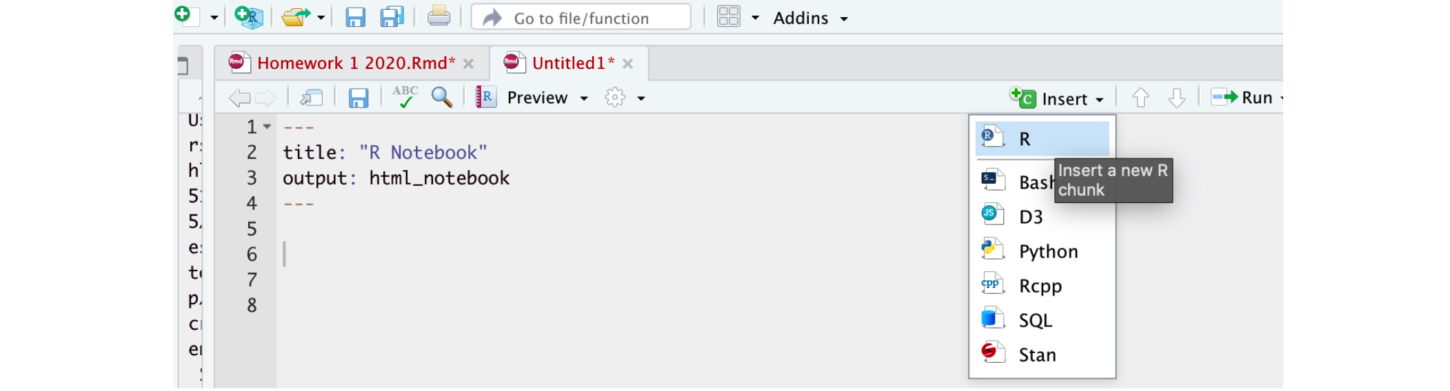
Now click at the end of the script, around line 20 and press the green insert button (top right in the script menu icons). Insert a new R code chunk. Inside, type 1+2 and run it. So you can see that you can have text/pictures/videos etc, and code chunks interspersed throughout it.

Now press the “knit” button (right next to the save button).

It will first ask you to save. Save it as STAT462_Lab1_PSU.ID e.g. STAT462_Lab1_hlg5155. Then, this should make a new file pop-up, a html pretty version of your code and output. If you go to your lab 1 folder, you will see that this has appeared next to your .Rmd file.

2.5.3 “Friendly text”

Much of what you see on your screen when you open a notebook document is simply a friendly introduction to RStudio.

So your notebook file is essentially a Word document with the ability to add in “mini R-consoles”, AKA your code chunks. Imagine every time you opened a new word document, it included some “friendly text” (“hi, this is a word document, this is how you do bold text, this is how you save”). This is great the first time you ever use Word, but kind of a pain after that.

RStudio actually does this. Every time you open a notebook file, you actually do get this friendly text, explaining how to use a notebook file. Read it, make sure you understand what it is telling you, then delete all of it. So delete from line 6 to the end. The stuff left over is your YAML code which tells R how to create the final html file. DON’T TOUCH THAT.

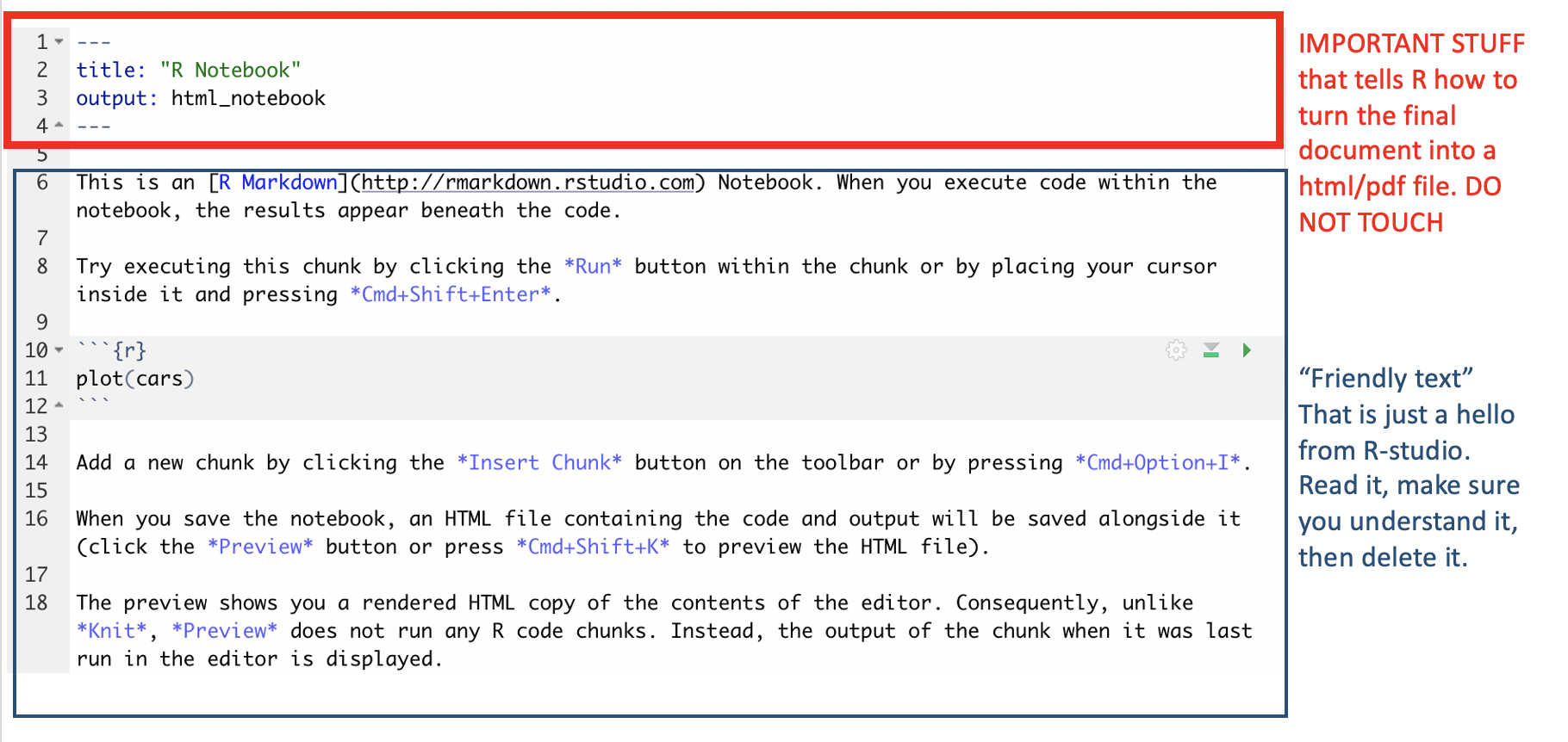
Figure 2.9: You should see TWO new files appear in your lab 1 folder

2.6 Lab Challenge 3

Your final challenge. In class we discussed about both numerical and graphical summaries to describe the data.You will be using the dataset mtcars available in R to make some numerical and graphical summaries.

NOTE: Don’t just copy paste the codes. Take a look at the help files for each of these functions and see of they make sense to you. You can also write notes to yourself about what the code does in the white text area of the R-notebook file.

Step 1:

Delete all the “friendly text” in your script - you should be just left with your YAML code and a blank file (see previous section)

Step 2:

We’re going to work with a table of data that’s already pre-loaded into R. First, type the ?mtcars command in the console. This will bring up the help file. Read the background of the dataset and briefly summarise it in your file (in the white space).

Step 3:

Click on the console and type View(mtcars). This should open a new tab where you can see a table showing the data. Have a look and get comfortable.

Now, create a code chunk by clicking on the Insert R-code button on the top right.

Type the lines of code below into the code chunk. Then run it by pressing the little green right arrow.

skim(mtcars)

This command compiles the summary statistics for the table you just saw. (you applied the skim command to the mtcars table). If this doesn’t work, make sure you installed and loaded the skimr library - or try the summary() command.

Below your code chunk,

You should be able to see that we’re dealing with a table with 11 columns that each tell us something about cars in 1974. Now answer the following questions, making sure to label them clearly in your text as a full sentence e.g. The median weight of the cars is…

Question A: What is the maximum value of the Gross horsepower of the cars?

Question B: What is the median weight of the cars.

If you are stuck, remember to read the help file from Step 2.

Step 4:

Suppose I want to compare the mileage of the vehicle for Auto and Manual transmission vehicles. We can make the comparison by making a side-by-side boxplot. Create a new code chunk. Use the code below to create the plot .

# boxplot is the command.  You can have a command on several lines.

boxplot(mpg~am,          # the miles per gallon column vs each level of transmission
        data=mtcars,                         # from the mtcars table
        xlab="Transmission",ylab="mpg", 
        names=c("Auto","Manual"),            # make nice labels
        col=c("deepskyblue4","deepskyblue")) # and colours

Question C: Briefly comment on what you can tell about the cars dataset from this plot.

Step 5:

As we discussed above, the mtcars table is loaded into R and we can look at it either by typing its name or by using commands like head() to show the first few lines.

But what if we want to access a specific column? This is where the $ symbol is useful. It means, “select the column named..”

For example if you type mtcars$cyl into the console, you will see that it just prints the data from the cyl column (number of cylinders) onto the screen. We could then apply a command to those numbers. For example mean(mtcars$cyl) will calculate the mean of all the values in the cyl column.

Question D: Create a new code chunk. Use the mean() and sd() commands to find the actual mean and standard deviation of the mpg column.

Once you have calculated these, under the code chunk, write a summary of your results as a full sentence e.g. The average miles-per-gallon of 1973-1974 car models was found to be…

Step 6:

We want to see if our data is normally distributed. We can do this using the histogram and normal-qq plot. The code below makes a histogram and QQNorm plot for the car horsepower. It also runs a Shapiro-Wilks test for the horsepower.

hist(mtcars$hp,br=10)

# The hash at the front of a line means I want R to ignore this code. It is invisible to R - a "comment"
# These two lines were the original way to make a QQ-norm plot. Feel free to uncomment and run them
# qqnorm(mtcars$mpg, pch = 1, frame = FALSE)
# qqline(mtcars$mpg, col = "steelblue", lwd = 2)

# Instead we are going to use a nicer format from the `ggpubr` library
ggqqplot(mtcars$hp,col="red")

# Shapiro Wilks test
shapiro.test(mtcars$hp)

## 
## 	Shapiro-Wilk normality test
## 
## data:  mtcars$hp
## W = 0.93342, p-value = 0.04881

Question E: In the text, in your own words, describe what a normal QQ-plot is and how to calculate one (if you’re not sure, do a google search - there are good videos!).

Question F: Run a histogram, Quantile-Quantile plot and a Shapiro-Wilks test for the MILES PER GALLON data. In the text below the plot write your conclusions about whether you are satisifed that a normal distribution can represent the miles per gallon data column and explain your reasoning.

Step 7:

Now we’re going to move onto some commands that allow us to calculate normal probabilities using R, rather than slowly by hand. Using the R functions pnorm() and qnorm(), we can find the cumulative probabilities and normal quantiles for any normal distribution.

For example, Cat lifespans have a normal distribution with a mean of 15.4 and a standard deviation of 2.3. What’s the probability of a cat lifespan less than 14 years?

?pnorm # use the help file of ?pnorm to see what lower.tail=TRUE/FALSE does
pnorm(14,mean=15.4,sd=2.4,lower.tail = TRUE)

## [1] 0.2798345

So, it’s 0.2798 - or ~28%

What about the probability of a cat being older than 20?

pnorm(20,mean=15.4,sd=2.4,lower.tail = FALSE)

## [1] 0.02764015

Normal quantiles go the other way around - they tell you the z score for whatever probability you require. For example, 80% of cats live to be what age?

qnorm(.80,mean=15.4,sd=2.4)

## [1] 17.41989

So the the answer is 17.42 years (remember the units!)

Question F:

Use R to find the probability below:

If X ∼ N(5,2), then find P(X ≤ 4)

Then Use R to find the value of the normal quantiles:

If X ∼ N(5,2), then find the value a such that P(X < a) = 0.025

Question H. Records maintained by the your admin office indicate that amount of time elapsed between the submission of travel receipts and the final reimbursement of funds has approximately a normal distribution with a mean of 39 days and a standard deviation of 6 days. If you submitted your travel claim 55 days ago, what is the probability that it should have been returned by now? What might you conclude?

Step 9:

Question I. In the text, explain to me something you didn’t already know about R

Step 10:

Question J. Finally, let’s include that project screenshot to learn that element of RMarkdown

Make sure the screenshot is in your Lab 1 folder. Now include a code chunk that looks similar to this, but with your user name/file name (note, it might be a .jpeg not a .png). When you run it, the screenshot should appear below the code chunk.

Step 11 OPTIONAL:

OPTIONAL Question K [BONUS 2%, lab capped at 100%]: Finally, if you would like your histograms and plots to look more professional, take a look at ggplot and see if you can make a histogram the mpg data using this approach instead. This is a good tutorial: https://www.r-graph-gallery.com/220-basic-ggplot2-histogram.html]

2.7 Submitting Lab 1 {Section.L1.7}

Remember to save your work throughout and to spell check your writing (next to the save button). Now, press the knit button again. If you have not made any mistakes in the code then R should create a new html file which includes your answers.

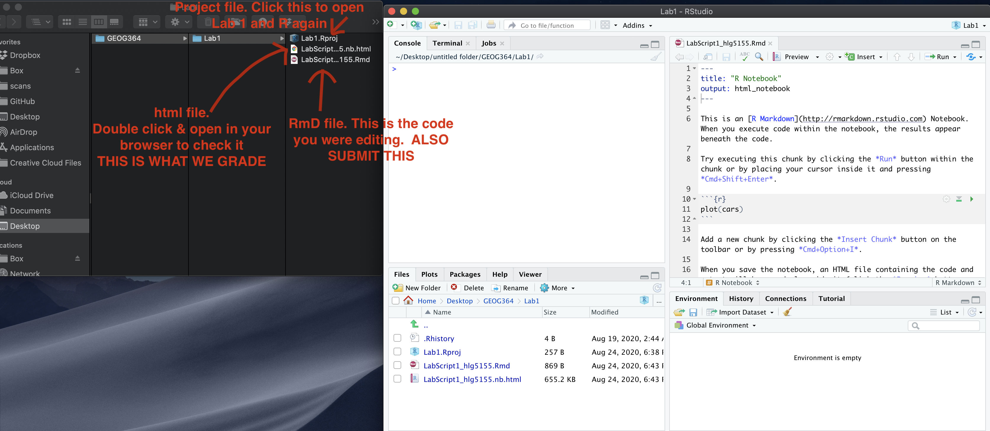
Figure 2.10: What you need to submit

If you look at your lab 1 folder, you should see this there - complete with a very recent time-stamp.

Now go to Canvas and submit BOTH your html and your .Rmd file in Lab 1.

2.7.1 Lab 1 submission check

MARKDOWN/CODE STYLE - 5 MARKS

Your code and document is neat and easy to read. LOOK AT YOUR HTML FILE IN YOUR WEB-BROWSER BEFORE YOU SUBMIT. There is also a spell check next to the save button.

WRITING STYLE - 5 MARKS

You have written your answers below the relevant code chunk in full sentences in a way that is easy to find and grade.

QUESTIONS A-D: 10 MARKS

You understand basic R commands and can describe the dataset

QUESTIONS E: 10 MARKS

10/10 for a detailed explanation I could provide to the class as an example (in your own words)
5/10 some attempt, but some clarification/tweaks would be needed
2/10 any attempt

QUESTIONS F: 10 MARKS

You can make and interpret a histogram, QQplot and a Wilks test for the MILES PER GALLON data

QUESTIONS G: 10 MARKS

You can calculate basic probabilities in R

QUESTION H: 20 MARKS

You can attempt a more lifelike question

QUESTION I: 10 MARKS

You engaged with the lab and can articulate your learning

QUESTION J: 10 MARKS

You can include a screenshot and are using projects correctly

HTML FILE SUBMISSION - 5 marks

RMD CODE SUBMISSION - 5 marks

[100 marks total]