Lab 1: Introduction to R
GEOG-364 - Spatial Analysis
GEOG-364 - Spatial Analysis
Dr Helen Greatrex
Dr Helen Greatrex
Welcome to Lab 1!
There are 8 labs in this course. Each one will build on the last one, with support provided in a series of tutorials (see the tutorials tab). You should NOT submit the tutorial work. We will work through the tutorials together and then your job is to submit the requirements on this page.
By the end of this week’s lab, you will be able to:
- Get comfortable with the lab format & how to work through them
- Know how to get help
- Get familiar with the RStudio interface
- Run your first programming commands
- Put everything together into an interactive markdown website (like this guide)
- Understand the process for submitting assignments
The lab is worth 110 points and there is a rubric at the end of this page.
Assignment 1 is due by midnight the night before your next lab on Canvas..
Step A: Tutorials
1. Set up R and R-Studio
- Read about R Tutorial 1A.
- Install BOTH R and R-Studio, or create an R-Studio Cloud account. This is covered in Tutorial 1B.
- Open R-Studio Make sure you click the right button!
- Set up your global settings. Work through Tutorial 2A and change your settings.
2. Getting set up for Lab 1
a. Projects
We are going to be storing each lab as a project. - Use Tutorial 2C - Projects to make your first R-project called GEOG364-Lab1-Project
a. Understanding the basics
Now we are going to take a look around and work through Tutorial 3 to get used to the console
c. Markdown basics
- Work through Tutorial 4A,4B and 4C to understand what R markdown is and to make your first Markdown document. You are going to make one as your lab report in the next section
d. Packages
Use Tutorial 2B - Libraries/Packages to understand what an R-Package is.
Now INSTALL these four packages. We will load them later on.
- tidyverse
- skimr
- ggplot2
- plotly
Step B: Actual lab
Everything above was for your own learning. Now we will start the actual lab you will submit:
1. Set up
Inside your R project, create a new RMarkdown document called
GEOG-364-Lab1.Rmd.Delete all the text below line 11 (e.g. everything from R Markdown onwards)
2. Packages
Now we need to load the packages we installed earlier on. (remember we only need to download the packages once, but we still need to load them every time we run our lab report (in the same way you only download your banking app once from the app store but need to press the icon every time you want to start using it). WE ALSO NEED TO LOAD THE PACKAGES IN A CODE CHUNK RATHER THAN IN THE CONSOLE. This is because When you press knit, in the background, your computer makes a new version of R where nothing is loaded, then it processes your code.
If you haven’t already, please first install them using the tutorial to help.
Then somewhere near the top of your script (but below the YAML code, so line 12 ish?), Create a code chunk. (if you’re stuck - https://rmarkdown.rstudio.com/lesson-3.html) and add this code.
library(skimr)
library(ggplot2)
library(plotly)- Run the code chunk! (pressing the green arrow, or go to the run button on the top right and press Run All). This will load the packages, Sometimes you see a load of “friendly loading text”. Try running the code chunk twice and it should go away.
3. Adding text to your report
In the white text area, create a level 1 heading called “Introduction to GEOG-364”. For a cheat sheet to help with this, move your mouse to the top of the page, click the help menu, then click Markdown Quick reference (spaces and whitespace are important!). If you want to add sub-headings etc, go for it!
Leave a blank line, then use the GEOG-364 syllabus to describe the course late policy in your own words (e.g. you’re writing about this in the white space).
Leave a blank line, then write how to contact Dr Greatrex and Yifei (e.g. e-mails vs canvas message? office hours?)
Press “knit” at the top of the screen. If you haven’t made a mistake a pop up should appear with a html file and your edits.
4. Adding maths and functions
Leave another blank line and add a new heading called “Code Showcase”. Add a blank line afterwards too. I say to leave a blank line because R ignores them and will tidy everything up. but if everything is scrunched up too close together (say you write text almost touching a code chunk), sometimes it works and sometimes it crashes annoyingly.
Create a code chunk .
INSIDE the code chunk, use R code to calculate the following (Hint, you can put these all in one code chunk, or have separate code chunks with them in. Just remember to leave blank lines between them)
1033 (e.g
103*103*103, or103^3)The square root of your age (google is your friend, google R command for square root)
Use R code to work out how many characters are in the longest town name in Wales Llanfairpwllgwyngyllgogerychwyrndrobwllllantysiliogogogoch.(Hint 1, remember you can copy paste this into your code. Hint 2.. remember your tutorials and quote marks!)
Create a sequence from 1000 to 2000, incrementing by 100 (e.g. 1000,1100,1200…). Hint, see what google says for R and sequences, or see here.
This should actually be running the code and showing you the answers in your document. If not, see https://rmarkdown.rstudio.com/lesson-3.html
Press “knit” at the top of the screen. If you haven’t made a mistake a pop up should appear with a html file and your edits. If you have made a mistake, the red text will tell you there is an error and which line it is on in your code. I’m happy to help debug.
5. Data analysis
Part 5 is taken from this tutorial (https://r4ds.had.co.nz/data-visualisation.html).
We’re going to work with a table of data that’s already pre-loaded
into R inside the ggplot2 package. Make sure you have run the library
code chunk. Now, type the ?mpg command in the console. This
will bring up the help file. If it can’t find the dataset, you need to
load the ggplot2 package using the library command or install
ggplot2.
a. Summarise the dataset.
Leave a blank line, and create a new heading called Car Analysis. Leave a blank line afterwards too. See above for why,
Read the background of the dataset in the help file and summarise it in your report (in the white space). E.g. imagine you are describing the dataset to a newspaper for a study.
b. Exploratory data analysis
Now look at the data itself. In the CONSOLE, type
View(mpg). This will open a new tab with the spreadsheet
itself.
Let’s look at the summary statistics. Leave a blank line and create a new code chunk containing the following code
# mpg comes from the ggplot2 package
summary(mpg)
or for the same thing but in a different format try
# mpg comes from the ggplot2 package
skim(mpg)
c. Your first plot
Let’s make your first scatter plot.
Among the variables in the mpg dataset are:
displ, a car’s engine size, in litres.hwy, a car’s fuel efficiency on the highway, in miles per gallon (mpg). A car with a low fuel efficiency consumes more fuel than a car with a high fuel efficiency when they travel the same distance.class, the class of car e.g. mini, SUV, pick up..
To make a nice looking plot of the relationship between these variables, create a code chunk, copy this code into it and run.
# ggplotly comes from the plotly package
# Choose the dataset and tell R the columns to plot
p <- ggplot(data = mpg) +
     geom_point(mapping = aes(x = displ, y = hwy, color = class))

ggplotly(p)  # Plot interactively
Now below your code, answer the following questions.
- What’s the object-of-analysis? (e.g. what does one row in the MPG SPREADSHEET/TABLE correspond to)
- Does this data tell me exactly how my personal car sitting outside my house will perform? Explain your answer.
- Create a code chunk and see if you can calculate the mean manufacturing year of the car models in the dataset.
- AS FULLY AS POSSIBLE BASED ON THE PLOT, describe the relationship between car’s engine size and its fuel efficiency on the highway. The more detail you add the more marks you get..
If you want to make it neat, you can use sub headings, or bold/italic text (see that R cheatsheet). Press knit a lot! Check you haven’t made a mistake, check it all works.
6. Version control AND… I WANT YOU TO CHEAT!
We believe that you did update/install R and R-studio, but given that there has recently been a huge spatial update and most issues come from the wrong version, we want to check
Create a new heading for this section & name it version control
Copy/paste this code into your lab script and run it. You should be on R version 4.4.1 (Race for Your Life) and RStudio 2024.04.2-“Chocolate Cosmos”. If not, go back to tutorial 1B or talk to Dr G.
##---###
# R Version
version

# R-Studio Version()
rstudioapi::versionInfo()
6b. Cheating???
The reason your homework was late is because I (Dr G) was coming up with a fancy new quiz structure. I want you to see if you can break it :)
https://aonsrp-helen-greatrex.shinyapps.io/quiz_template/
Try the quiz a few times, getting it wrong first a few times then right. When they are all correct, you will see a unique pass-code.
Copy/paste it to a code chunk that looks like this in your lab report and replace “word1-word2” with your password
password <- "word1-word2"BONUS MARKS! NOW….. I WANT YOU TO BREAK MY QUIZ!! FOR EXAMPLE THERE ARE 10000 passcodes and the questions/answers out there, try to find them, or think of every way someone could cheat this. The actual quiz will have infinitely rotating questions.
If you find the the codes/questions/answers and show me how you do it, you automatically get 100% on lab 1.
7. Above and beyond
Remember that an A is 94%, so you can ignore this section and still easily get an A.
But here is your time to shine. Also, if you are struggling in another part of the lab, you can use this to gain back points.
To get the final 5 marks in the lab, you need to show me someting new, e.g. you need to go above and beyond the lab questions in some way.
- You get 2/5 for doing something new in any way sliding scale to..
- You get 5/5 for something really impressive or multiple small things.
Please tell us in your R script what you did!
Here in lab 1, maybe you added in different text formats to make your
lab script more clear (bold/italic etc). Maybe you worked out how to add
axis labels to ggplot (note, it’s a pain), maybe you used nested
headings or sub-headings, or worked out how to add a table of
contents.
Or.. ask chatgpt to make you a cool plot with the mpg data. Or check out
the ggstatplot package.
C. Submitting your Lab
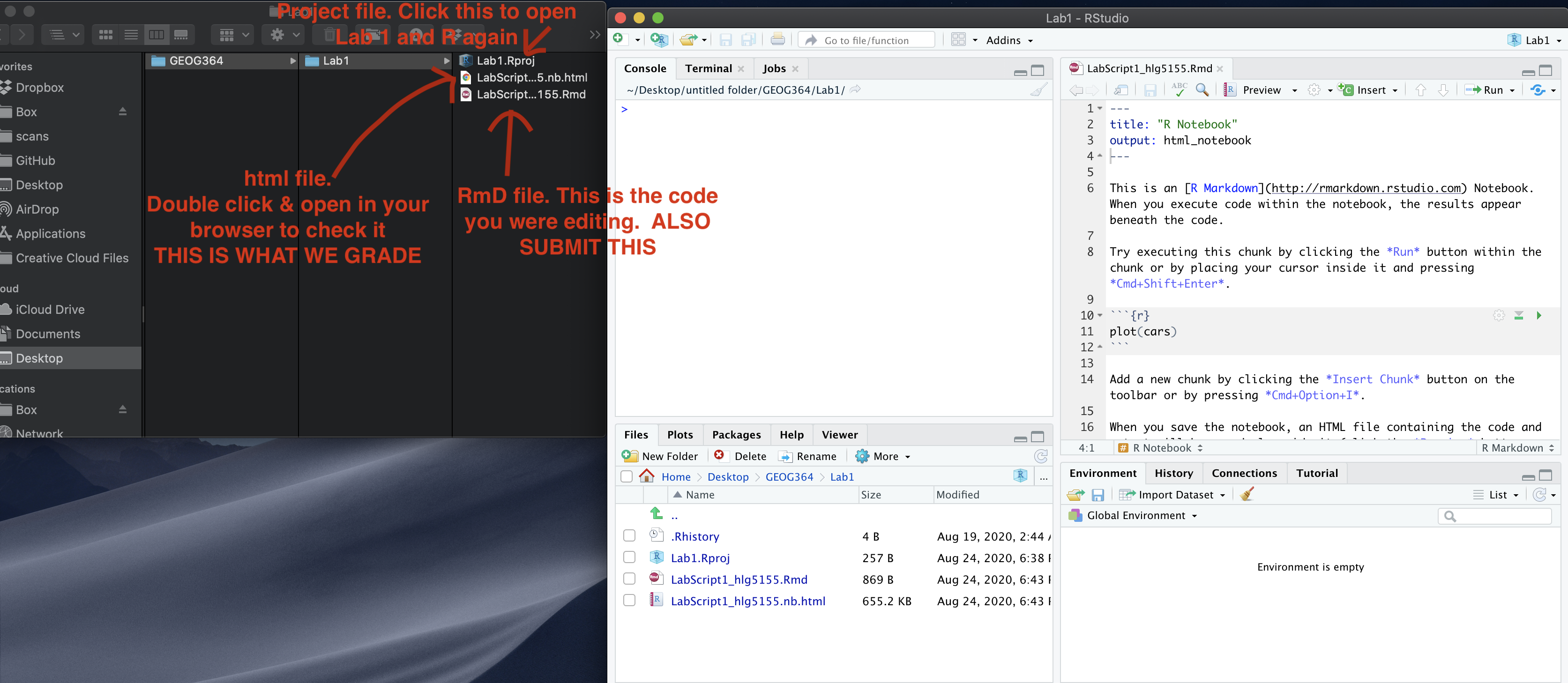
Remember to save your work throughout and to spell check your writing (next to the save button). Now, press the knit button again. If you have not made any mistakes in the code then R should create a html file in your lab 1 folder which includes your answers. If you look at your lab 1 folder, you should see this there - complete with a very recent time-stamp.
In that folder, double click on the html file. This will open it in your browser. CHECK THAT THIS IS WHAT YOU WANT TO SUBMIT
Now go to Canvas and submit BOTH your html and your .Rmd file in Lab 1.
Lab 1 submission check-list
HTML FILE SUBMISSION - 10 marks
RMD CODE SUBMISSION - 10 marks
MARKDOWN/CODE STYLE - 20 MARKS
Your code and document is neat and easy to read. LOOK AT YOUR HTML FILE IN YOUR WEB-BROWSER BEFORE YOU SUBMIT. There is also a spell check next to the save button. You have written your answers below the relevant code chunk in full sentences in a way that is easy to find and grade. For example, you have written in full sentences, it is clear what your answers are referring to.
Introduction to GEOG-364: 15 MARKS
You have described the lab late policy clearly in a way I could share with a new student.
Code Showcase: 20 MARKS
You have managed to successfully complete all the code challenges
Car analysis: 25 MARKS
You included all the code and successfully answered the questions, providing reasoning where appropriate
Versions: 5 MARKS
You included the code showing your version AND it was the most up to date version of R AND R-STUDIO
Above and beyond: 5 MARKS
Here you need to go above and beyond the lab questions in some way. Here in lab 1, maybe you added in different text formats to make your lab script more clear (bold/italic etc). Maybe you worked out how to add axis labels to ggplot (note, it’s a pain), maybe you used nested headings or sub-headings, or worked out how to add a table of contents.
You get 2/5 for doing something new in any way, scaled to 5/5 for something really impressive or multiple small things.
[110 marks total]
Overall, here is what your lab should correspond to:
| Grade | % Mark | Rubric |
|---|---|---|
| A* | 98-100 | Exceptional. Not only was it near perfect, but the graders learned something. THIS IS HARD TO GET. |
| NA | 96+ | You went above and beyond |
| A | 93+: | Everything asked for with high quality. Class example |
| A- | 90+ | The odd minor mistake, All code done but not written up in full sentences etc. A little less care |
| B+ | 87+ | More minor mistakes. Things like missing units, getting the odd question wrong, no workings shown |
| B | 83+ | Solid work but the odd larger mistake or missing answer. Completely misinterpreted something, that type of thing |
| B- | 80+ | Starting to miss entire/questions sections, or multiple larger mistakes. Still a solid attempt. |
| C+ | 77+ | You made a good effort and did some things well, but there were a lot of problems. (e.g. you wrote up the text well, but messed up the code) |
| C | 70+ | It’s clear you tried and learned something. Just attending labs will get you this much as we can help you get to this stage |
| D | 60+ | You attempt the lab and submit something. Not clear you put in much effort or you had real issues |
| F | 0+ | Didn’t submit, or incredibly limited attempt. |
Website created and maintained by Helen Greatrex. Website template by Noli Brazil