1 Reading in data

2 Summary Statistics

2.1 Introduction

Before analyzing a dataset, it’s essential to understand its structure, size, and data types. It is then often useful to understand more about the data inside to help with quality control.

Suggested libraries

library(dplyr)
library(skimr)
library(GGally)

The tutorial is based on a small test dataset with four columns:

Make (categorical)
MPG (numerical)
Cylinders (categorical)
Transmission (categorical)

# Create a simple dataset with numerical and categorical variables
test_data <- data.frame(
  Make = factor(c("Toyota", "Ford", "Honda", "Chevy", "Nissan", "BMW")),
  MPG = c(30, 25, 27, 22, 29, 24),
  Cylinders = factor(c(4, 6, 4, 8, 4, 6)),
  Transmission = factor(c("Auto", "Manual", "Auto", "Auto", "Manual", "Manual"))
)

2.2 Assessing data structure

Before analyzing a dataset, it’s essential to understand its structure, size, and data types. This tutorial will guide you through:

Viewing the dataset.
Checking its dimensions, column names, and structure.
Understanding data types and modifying them if necessary.
Preparing for summary statistics.

2.2.1 Viewing Data

To explore the dataset interactively, you can:

Open it in the RStudio Data Viewer:
Run View(test_data) in the console.
Note: View() should not be placed inside a code chunk because it only works interactively in RStudio and does not produce console output. It often breaks the knitting process
See a tabular preview in the environment pane:
Click on test_data in the environment tab.
Print the entire dataset (not recommended for large datasets):

test_data

##     Make MPG Cylinders Transmission
## 1 Toyota  30         4         Auto
## 2   Ford  25         6       Manual
## 3  Honda  27         4         Auto
## 4  Chevy  22         8         Auto
## 5 Nissan  29         4       Manual
## 6    BMW  24         6       Manual

View only the first few rows:

head(test_data)

##     Make MPG Cylinders Transmission
## 1 Toyota  30         4         Auto
## 2   Ford  25         6       Manual
## 3  Honda  27         4         Auto
## 4  Chevy  22         8         Auto
## 5 Nissan  29         4       Manual
## 6    BMW  24         6       Manual

2.2.2 Column Names

To see what columns exist:

names(test_data)

## [1] "Make"         "MPG"          "Cylinders"    "Transmission"

2.2.3 Number of Rows/Columns

To find out how many rows and columns there are:

nrow(test_data)  # Number of rows

## [1] 6

ncol(test_data)  # Number of columns

## [1] 4

dim(test_data)   # Dimensions (rows, columns)

## [1] 6 4

2.2.4 General Structure

To get a compact summary of the dataset, str() provides an overview, including the number of observations, variables, and data types.

str(test_data)

## 'data.frame':    6 obs. of  4 variables:
##  $ Make        : Factor w/ 6 levels "BMW","Chevy",..: 6 3 4 2 5 1
##  $ MPG         : num  30 25 27 22 29 24
##  $ Cylinders   : Factor w/ 3 levels "4","6","8": 1 2 1 3 1 2
##  $ Transmission: Factor w/ 2 levels "Auto","Manual": 1 2 1 1 2 2

Another alternative is glimpse() (from dplyr):

glimpse(test_data)

## Rows: 6
## Columns: 4
## $ Make         <fct> Toyota, Ford, Honda, Chevy, Nissan, BMW
## $ MPG          <dbl> 30, 25, 27, 22, 29, 24
## $ Cylinders    <fct> 4, 6, 4, 8, 4, 6
## $ Transmission <fct> Auto, Manual, Auto, Auto, Manual, Manual

2.2.5 Data-type/Grouped Data

Each column in a dataset has a specific data type (e.g., numeric, character, factor). “Factor” is the R jargon for variables that have a fixed number of unique values (e.g., categories/groups/families).

We can check the data types using:

sapply(test_data, class)

##         Make          MPG    Cylinders Transmission 
##     "factor"    "numeric"     "factor"     "factor"

If categorical variables are not stored as factors, we can explicitly define them:

test_data$Cylinders <- factor(test_data$Cylinders, levels = c(4, 6, 8))
test_data$Transmission <- factor(test_data$Transmission, levels = c("Auto", "Manual"))

This ensures:

Consistent ordering of categorical levels.
Avoiding unintended sorting in plots or models.

Similarly, if data “should” be numeric, but isn’t for some reason, we can convert it using as.numeric() etc.

2.3 Summary Statistics

Summary statistics are a way to summarize the main characteristics of the data inside a dataset. They can be used to describe the central tendency, dispersion, and shape of a dataset’s distribution.

2.3.1 General summary functions

We can use the summary() function to get a quick overview of numerical variables.

summary(test_data)

##      Make        MPG        Cylinders Transmission
##  BMW   :1   Min.   :22.00   4:3       Auto  :3    
##  Chevy :1   1st Qu.:24.25   6:2       Manual:3    
##  Ford  :1   Median :26.00   8:1                   
##  Honda :1   Mean   :26.17                         
##  Nissan:1   3rd Qu.:28.50                         
##  Toyota:1   Max.   :30.00

Alternatively, we can calculate specific summary statistics manually using base R and dplyr.

# Using base R
mean(test_data$MPG)  # Mean MPG

## [1] 26.16667

median(test_data$MPG) # Median MPG

## [1] 26

sd(test_data$MPG)     # Standard deviation

## [1] 3.060501

range(test_data$MPG)  # Minimum and maximum

## [1] 22 30

# Using dplyr
test_data %>%
  summarise(
    Mean_MPG = mean(MPG),
    Median_MPG = median(MPG),
    SD_MPG = sd(MPG),
    Min_MPG = min(MPG),
    Max_MPG = max(MPG)
  )

##   Mean_MPG Median_MPG   SD_MPG Min_MPG Max_MPG
## 1 26.16667         26 3.060501      22      30

There are also specific summary commands from a variety of packages including

2.3.1.1 Enhanced Summaries with `skimr`

The skimr package provides an easy and readable summary of the dataset.

skim(test_data)

Data summary
Name	test_data
Number of rows	6
Number of columns	4
_______________________
Column type frequency:
factor	3
numeric	1
________________________
Group variables	None

Variable type: factor

skim_variable	complete_rate	ordered	n_unique	top_counts
Make	1	FALSE	6	BMW: 1, Che: 1, For: 1, Hon: 1
Cylinders	1	FALSE	3	4: 3, 6: 2, 8: 1
Transmission	1	FALSE	2	Aut: 3, Man: 3

Variable type: numeric

skim_variable	n_missing	complete_rate	mean	sd	p0	p25	p50	p75	p100	hist
MPG	0	1	26.17	3.06	22	24.25	26	28.5	30	▃▇▁▃▇

2.3.1.2 Pairwise Relationships with `GGally`

The GGally package provides useful visual summaries of numerical variables.

if (!require(GGally)) install.packages("GGally", dependencies = TRUE)
library(GGally)
# Create pairwise scatter plots
GGally::ggpairs(test_data, columns = c("MPG"))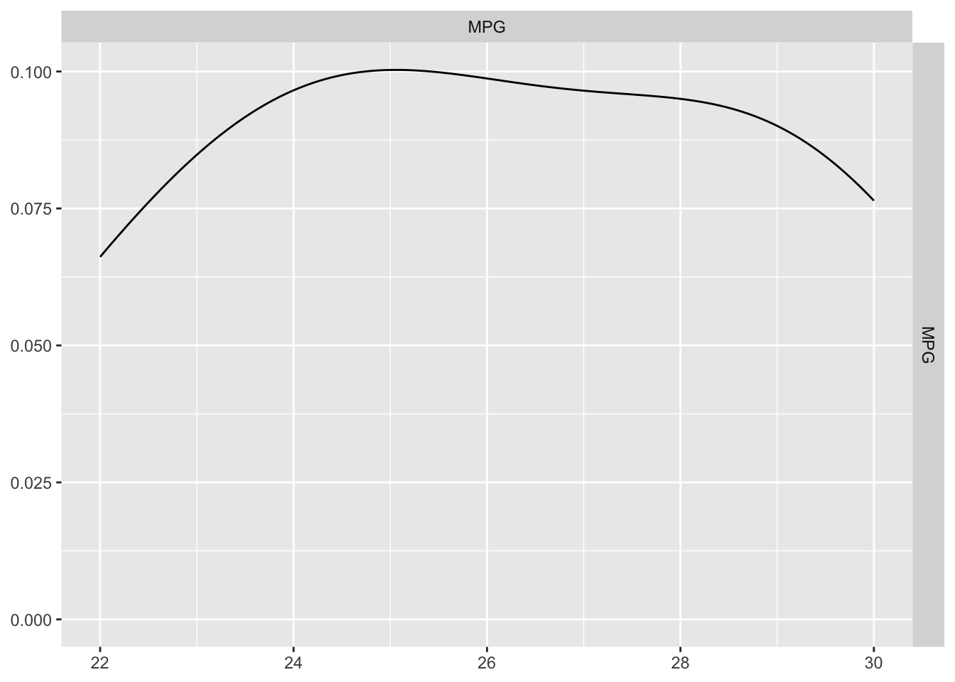

2.3.2 Frequency tables

We can use table() or dplyr::count() to summarize categorical variables. e.g. count how many rows there are in different categories. This is especially useful for categorical data.

The easiest way to do this is using the table command. For example to see how many cars have each type of transmission:

table(test_data$Transmission)

## 
##   Auto Manual 
##      3      3

So there are three rows with automatic cars and three with manual, We can also make two way tables

table(test_data$Transmission, test_data$Cylinders)

##         
##          4 6 8
##   Auto   2 0 1
##   Manual 1 2 0

So there are 2 cars that are automatic with four cylinders. We can also use the count function in dplyr

test_data %>% count(Transmission)

##   Transmission n
## 1         Auto 3
## 2       Manual 3

2.3.3 Grouped Summary Statistics

We can also compute statistics such as the mean, maximum, and minimum values for different groups.

Tidyverse Approach

Using group_by() and summarise(), we can compute statistics for each species:

test_data %>%
  group_by(Transmission) %>%
  summarise(
    Mean_MPG = mean(MPG),
    Median_MPG = median(MPG),
    Count = n()
  )

## # A tibble: 2 × 4
##   Transmission Mean_MPG Median_MPG Count
##   <fct>           <dbl>      <dbl> <int>
## 1 Auto             26.3         27     3
## 2 Manual           26           25     3

Base R Approach

I admit, tidyverse is better in this case!

aggregate(cbind(MPG, MPG) ~ Transmission, data = test_data, 
          FUN = function(x) c(mean = mean(x, na.rm = TRUE), max = max(x, na.rm = TRUE)))

##   Transmission MPG.mean  MPG.max MPG.mean  MPG.max
## 1         Auto 26.33333 30.00000 26.33333 30.00000
## 2       Manual 26.00000 29.00000 26.00000 29.00000

3 Filtering/Selecting

4 Data Wrangling

4.1 Introduction & packages

This tutorial explains how to filter, select, summarize, and wrangle data in R using both Tidyverse and Base R approaches.

Both approaches are valid, but they differ in syntax and philosophy. Tidyverse functions (from dplyr) use a pipeline-based approach, whereas Base R relies on indexing and built-in functions.

# Load necessary packages
library(tidyverse)  # Core data wrangling
library(palmerpenguins) # Example dataset
library(skimr)  # Quick summary stats
library(GGally)  # Pair plots
library(ggplot2) # Visualization

We will use the penguins dataset from the palmerpenguins package to demonstrate data wrangling techniques.

data("penguins")  # Load dataset

4.2 Selecting Data

4.2.1 Selecting a specific column using $

Sometimes we want to deal with only one specific column in our dataset, for example applying the mean command to say just one column.

To do this, we use the $ symbol. For example, here I’m simply selecting the data in the elevation column only and saving it to a new variable called elevationdata.

mean_mass <- penguins$body_mass_g 

mean_mass

Try it yourself. You should have seen that as you typed the $, it gave you all the available column names to choose from. This means we can now easily summarise specific columns. For example:

summary(penguins) will create a summary of the whole spreadsheet,
summary(penguins$Price) will only summarise the Price column.
mean(penguins$Price) will take the mean of the Price column in the HousesNY dataframe.

4.2.2 Selecting multiple columns

Remember you have the names() command to help find these and that the names are CASE SENSITIVE. If we want to work with several specific columns (e.g., species, bill_length_mm, and flipper_length_mm), we can extract them like this:

Tidyverse Approach

selected_data <- penguins %>% dplyr::select(species, bill_length_mm, flipper_length_mm)
head(selected_data)

## # A tibble: 6 × 3
##   species bill_length_mm flipper_length_mm
##   <fct>            <dbl>             <int>
## 1 Adelie            39.1               181
## 2 Adelie            39.5               186
## 3 Adelie            40.3               195
## 4 Adelie            NA                  NA
## 5 Adelie            36.7               193
## 6 Adelie            39.3               190

Base R Approach

selected_data <- penguins[, c("species", "bill_length_mm", "flipper_length_mm")]
head(selected_data)

## # A tibble: 6 × 3
##   species bill_length_mm flipper_length_mm
##   <fct>            <dbl>             <int>
## 1 Adelie            39.1               181
## 2 Adelie            39.5               186
## 3 Adelie            40.3               195
## 4 Adelie            NA                  NA
## 5 Adelie            36.7               193
## 6 Adelie            39.3               190

4.2.3 Selecting specific values

Sometimes, we do not want to analyse at the entire data.frame. Instead, we would like to only look at one (or more) columns or rows.

There are several ways we can select data.

To choose a specific column, we can use the $ symbol to select its name (as described above)
If you know which number rows or columns you want, you can use square brackets to numerically select data. Essentially our data follows the matrix format format:

\[ tablename [ ROWS , COLUMNS ] \]

Some examples:

# This will select the data in the 5th row and 7th column
penguins[5,7]

# This will select the 2nd row and ALL the columns 
penguins[2,]

# This will select the 3rd column and ALL the rows
penguins[,3]
# similar to using its name
penguins$island

# We can combine our commands, this will print the 13th row of the body mass column 
# (no comma as we're only looking at one column)
penguins$body_mass_g[13] 

# The : symbol lets you choose a sequence of numbers e.g. 1:5 is 1 2 3 4 5
# So this prints out rows 11 to 15 and all the columns
penguins[11:15,]

# The "c" command allows you to enter whatever numbers you like.  
# So this will print out rows 4,3,7 and the "Elevation" and "Dist_to_Coast" columns
penguins[c(4,3,7), c("island","body_mass_g")]

4.2.4 Deleting data

Or if you know the row or column number you can use the minus - sign to remove. Or use filter..

# remove row 6 and and overwrite
penguins <- penguins[-6 ,]

# remove columns 4 and 2 and save result to newdata 
newdata <- penguins[, - c(2,4) ]

4.3 Filtering rows

Filtering means selecting only the rows that meet certain conditions.

which() helps find row numbers that match a condition.
filter() (from dplyr tidyverse) allows for clear, intuitive filtering of data.
Logical operators (&, |, !=, %in%) provide additional flexibility in specifying conditions.

4.3.1 BaseR `which()` command

The which() command helps us identify row indices that meet a condition.

For example, identifying numbers greater than 107 in a sequence:

a <- 100:110
which(a > 107)

I like it because you can read the command as a sentence e.g. which numbers in “a” are greater than 107, Or which penguins have a body_mass_g less than or equal to 3000g:

outlier_rows <- which(penguins$body_mass_g <= 3000)

To find the row corresponding to the penguin with the smallest bill length:

row_number <- which(penguins$bill_length_mm == min(penguins$bill_length_mm, na.rm = TRUE))
smallest_bill <- penguins[row_number, ]
smallest_bill

4.3.2 Tidyverse/dplyr filter command

We can also use the tidyverse approach, the dplyr::filter() function. All the condition symbols e.g. !=NOT etc also work for the which command,

Selecting all Adelie penguins:

filter(penguins, species == "Adelie")

Selecting multiple species using %in%:

filter(penguins, species %in% c("Adelie", "Chinstrap"))

Excluding a species using !=:

filter(penguins, species != "Gentoo")

Filtering penguins with a flipper length greater than 200 mm:

filter(penguins, flipper_length_mm > 200)

Filtering penguins with a body mass less than or equal to 3000 g:

light_penguins <- filter(penguins, body_mass_g <= 3000)
summary(light_penguins)

Filtering with multiple conditions:

filter(penguins, flipper_length_mm > 180 & species == "Adelie")

Using | (OR condition) to select penguins with either a bill_depth_mm greater than 18 or flipper_length_mm longer than 210 mm:

filter(penguins, bill_depth_mm > 18 | flipper_length_mm > 210)

4.4 Saving data to new columns

Lets say you wanted to find the ratio between two columns of data, then save your answer as a new column

Base R Approach

penguins$bill_ratio <- penguins$bill_length_mm / penguins$bill_depth_mm

Tidyverse Approach

penguins <- penguins %>% mutate(bill_ratio = bill_length_mm / bill_depth_mm)

4.5 Sorting Data

Sorting the data allows us to find the highest and lowest values in a dataset.

Sort by body mass (ascending):

Tidyverse Approach

penguins <- arrange(penguins, body_mass_g)

Sort by descending order:

penguins <- arrange(penguins, desc(flipper_length_mm))

Base R Approach

penguins <- penguins[order(penguins$body_mass_g), ]

penguins <- penguins[order(-penguins$flipper_length_mm), ]

4.6 Combining Everything

We can combine multiple operations into a single pipeline. The tidyverse is designed for this.

Tidyverse Approach

final_result <- penguins %>%
  filter(flipper_length_mm > 180) %>%
  mutate(bill_ratio = bill_length_mm / bill_depth_mm) %>%
  select(species, bill_length_mm, flipper_length_mm, bill_ratio) %>%
  arrange(desc(bill_ratio))

Base R Approach

filtered <- penguins[penguins$flipper_length_mm > 180, ]
filtered$bill_ratio <- filtered$bill_length_mm / filtered$bill_depth_mm

filtered <- filtered[order(-filtered$bill_ratio),
                     c("species", "bill_length_mm", 
                       "flipper_length_mm", "bill_ratio")]
head(filtered)

5 Missing data

5.1 All the commands

Before starting, ensure you have these packages installed and loaded:

library(skimr)   # For detailed data summaries
library(dplyr)   # For data manipulation
library(naniar)  # For missing data visualization
library(tidyr)   # Lots of useful functions for data cleaning

Here are the commands covered in this guide to make it easy to copy/paste. Remember to replace testdata with the name of your dataset - and keep reading for what each command does.

#-------------------------------------------
# Visualizing Missing Data
#-------------------------------------------
summary(testdata)        # Summary statistics
skim(testdata)           # Skim summary (detailed)
colSums(is.na(testdata)) # Count NAs per column
rowSums(is.na(testdata)) # Count NAs per row
sum(is.na(testdata$x))   # Count NAs in column x
gg_miss_var(testdata)    # naniar: Missing values per variable
vis_miss(testdata)       # naniar: Heatmap of missing values

#-------------------------------------------
# Removing Rows with Missing Data
#-------------------------------------------
data_complete <- na.omit(testdata)
data_filtered <- testdata %>% dplyr::filter(!is.na(x) & !is.na(z)) 

# using tidyr
testdata <- testdata %>% replace_na(list(x = 0, y = "Unknown"))
testdata <- testdata %>% drop_na(x, y)  

#-------------------------------------------
# Replacing missing values. In this case
# Replace NAs with 99
#-------------------------------------------
testdata$x <- ifelse(is.na(testdata$x), 99, testdata$x)  


#-------------------------------------------
# Handling NAs in Common Functions
#-------------------------------------------
meanx <- mean(testdata$x, na.rm=TRUE)   
sdx <- sd(testdata$x, na.rm=TRUE)       
table(testdata$y, useNA = "ifany")       
cor(testdata, use = "pairwise.complete.obs")  
lm(z ~ x, data = testdata, na.action = na.omit)    # Omitting NAs
lm(z ~ x, data = testdata, na.action = na.exclude) # Keeping track of NAs, prefer

5.2 What is Missing Data

Before making decisions about how to handle missing data, you need to identify where it’s present. In R, NA represents missing values. You might also encounter NaN (Not a Number), which is another type of missing value.

Many ways of writing ‘missing’

When reading in external datasets, missing values may be represented differently. Common placeholders include:

-1 (often used in government datasets)
99, -99, 9999, 999 (arbitrary placeholders for missing values)
Blank cells in spreadsheets

5.2.1 There are different types of missing

Understanding why data is missing is crucial before deciding how to handle it:

Missing Completely at Random (MCAR)
- The probability of missingness is unrelated to any variable in the dataset.
- Example: A sensor randomly fails.
Missing at Random (MAR)
- Missingness is related to observed data but not the missing values themselves.
- Example: Younger participants are less likely to report their income, but within each age group, missingness is random.
Missing Not at Random (MNAR)
- Missingness depends on the value of the missing data itself.
- Example: People with higher incomes are less likely to report their income.

Key Takeaways: - If data is MCAR, deleting missing cases is often unbiased. - If data is MAR, multiple imputation methods may help recover missing values. - If data is MNAR, the missingness mechanism itself needs to be modeled.

5.3 Files with missing data

If you know your dataset uses non-standard missing value indicators, you can explicitly define them when reading in the data. No matter what, check the data carefully to make sure you didn’ make a mistake.

CSV Files

data <- read.csv("data.csv", na.strings = c("", "NA", "-1", "99", "9999"))

na.strings tells R which values should be treated as NA.
This example converts empty strings (""), standard NA, -1, 99, and 9999 into missing values.

Excel files

library(readxl)
data <- read_excel("data.xlsx", na = c("", "NA", "-1", "999"))

na defines missing values similarly to na.strings in read.csv().

Reading Data with `tidyverse` (readr package)

library(readr)
data <- read_csv("data.csv", na = c("", "NA", "-1", "999"))

read_csv() is part of tidyverse and often preferred for faster performance and better defaults.

5.4 Summarising Missing Data

Before deciding how to handle missing data, it’s crucial to first identify where it’s present. Let’s create a small dataset with missing values. The final column includes many empty values to mimic real-world data.

testdata <- data.frame(
  x = c(1, 2, 3, NA, 5),
  y = c("A", "B", "C", "D", NA),
  z = c(10, 15, NA, 20, 25),
  randomnotes = c(NA, NA, NA, "hello", NA)
)
print(testdata)

##    x    y  z randomnotes
## 1  1    A 10        <NA>
## 2  2    B 15        <NA>
## 3  3    C NA        <NA>
## 4 NA    D 20       hello
## 5  5 <NA> 25        <NA>

along with example outputs. I apply everything to the basic test data above.

General Summaries

Summary functions provide an overview of missing data:

summary(testdata)  # Basic summary statistics

##        x             y                   z         randomnotes       
##  Min.   :1.00   Length:5           Min.   :10.00   Length:5          
##  1st Qu.:1.75   Class :character   1st Qu.:13.75   Class :character  
##  Median :2.50   Mode  :character   Median :17.50   Mode  :character  
##  Mean   :2.75                      Mean   :17.50                     
##  3rd Qu.:3.50                      3rd Qu.:21.25                     
##  Max.   :5.00                      Max.   :25.00                     
##  NA's   :1                         NA's   :1

skim(testdata)     # More detailed summary, including missing values

Data summary
Name	testdata
Number of rows	5
Number of columns	4
_______________________
Column type frequency:
character	2
numeric	2
________________________
Group variables	None

Variable type: character

skim_variable	n_missing	complete_rate	min	max	empty	n_unique	whitespace
y	1	0.8	1	1	0	4	0
randomnotes	4	0.2	5	5	0	1	0

Variable type: numeric

skim_variable	n_missing	complete_rate	mean	sd	p0	p25	p50	p75	p100	hist
x	1	0.8	2.75	1.71	1	1.75	2.5	3.50	5	▇▇▇▁▇
z	1	0.8	17.50	6.45	10	13.75	17.5	21.25	25	▇▇▁▇▇

Visualizing NA numbers (naniar package)

The naniar package provides helpful visualizations. Install and load it before use.

gg_miss_var(testdata)  # Missing values per variable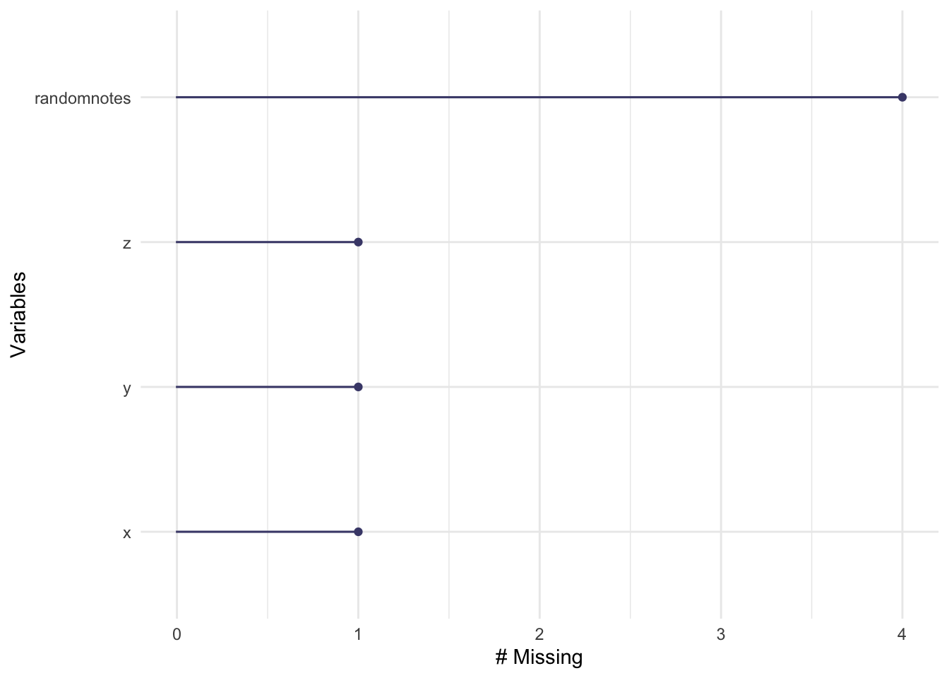

vis_miss(testdata)     # Heatmap of missing values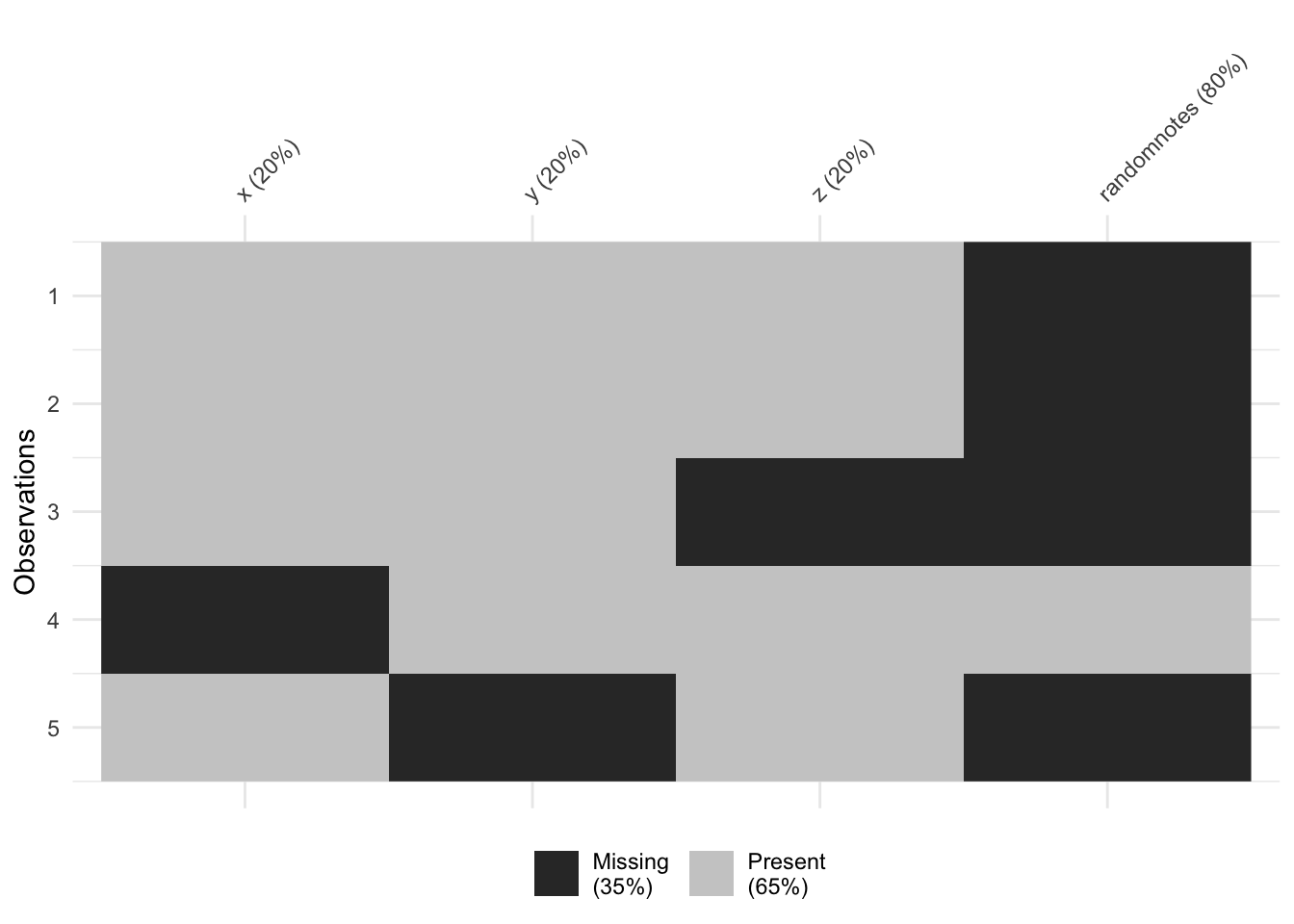

Counting NAs

You can count missing values at different levels:

colSums(is.na(testdata))            # Count NAs per column

##           x           y           z randomnotes 
##           1           1           1           4

rowSums(is.na(testdata))            # Count NAs per row

## [1] 1 1 2 1 2

sum(is.na(testdata$x))              # Count NAs in a specific column

## [1] 1

# Frequency table including missing values
table(testdata$y, useNA = "ifany")

## 
##    A    B    C    D <NA> 
##    1    1    1    1    1

5.5 Handling Missing Data

Missing data can cause errors in analyses, so it is often necessary to handle it appropriately. Removing missing data is only advisable when the data is Missing Completely at Random (MCAR).

1. Remove entire row if NA present

Listwise deletion, or Complete Case Analysis, removes entire rows if any column contains missing data. This can significantly reduce your dataset, so use it with caution.

data_complete <- na.omit(testdata)  # Remove rows with any NA

# Check for potential bias introduced by removal:
summary(data_complete)

##        x            y                   z       randomnotes       
##  Min.   : NA   Length:0           Min.   : NA   Length:0          
##  1st Qu.: NA   Class :character   1st Qu.: NA   Class :character  
##  Median : NA   Mode  :character   Median : NA   Mode  :character  
##  Mean   :NaN                      Mean   :NaN                     
##  3rd Qu.: NA                      3rd Qu.: NA                     
##  Max.   : NA                      Max.   : NA

Warning: If many columns have missing data (especially ones you don’t care about, such as “notes”), then this method may remove too many observations. For example in this case, I removed most of my valuable information.

2. Removing Rows with NAs in Chosen Columns

If you want to only remove rows with missing values in a single column, we can use the complete cases command. E.g. take the testdata table and ONLY include objects that are not missing their x-value. Note, this can be any column name at all.

data_filtered <- testdata[complete.cases(testdata$x), ]

You can also do this manually using filter and the is.na() command

# Tidyverse
data_filtered <- testdata %>% 
  dplyr::filter(!is.na(x) & !is.na(z))

# BaseR
data_filtered <- testdata[which(!is.na(testdata$x) & !is.na(testdata$z)), ]

5.5.1 3. Turning values into NA

Sometimes, you have -999 or something as your missing datacode and you missed it reading in the data. You can also use the filter command to force data to be NA.

E.g. here I select all the prices in a house dataset that are less than 0 (e.g impossible) and set them to NA.

HousesNY$Price[HousesNY$Price < 0]   <- NA

E.g. here I select all the prices that are less than 0 (e.g impossible) and set them to NA.

3. Replace NAs with data

This is useful when you want to keep the row but replace the missing value with a specific number.

testdata$x <- ifelse(is.na(testdata$x), 99, testdata$x)  # Replace NAs with 99

4. Use the `tidyr` package

The tidyr package provides a more elegant way to replace NAs. Remember to load/install it first!

Using tidyr::replace_na()

testdata <- testdata %>% replace_na(list(x = 0, y = "Unknown"))

Filtering Out NAs Using drop_na() (tidyr)

testdata <- testdata %>% drop_na(x, y)  # Removes rows where x or y is NA

5.6 Common Functions & NAs

You don’t always have to remove missing data in advance. Many R functions allow you to handle missing values within the function itself, preventing unnecessary data loss. The best way to check if a function has an option for handling missing values is to look at its help file using ?function_name.

5.6.1 The na.rm() option in commands.

If there is missing data, then by default, R will set the answer to any statistics to also be missing.

Remember this is our test data

print(testdata)

##    x       y  z randomnotes
## 1  1       A 10        <NA>
## 2  2       B 15        <NA>
## 3  3       C NA        <NA>
## 4 99       D 20       hello
## 5  5 Unknown 25        <NA>

Taking the mean of z results in NA

# Take the mean of column B
mean(testdata$z)

## [1] NA

# Take the correlation between A and B
cor(testdata$x,testdata$z)

## [1] NA

But many commands include an option (often na.rm=TRUE) which you can add to ignore missing data

# na.rm  e.g. remove NAs = TRUE
mean(testdata$z, na.rm=TRUE)

## [1] 17.5

sd(testdata$z, na.rm=TRUE)

## [1] 6.454972

or sometimes I look in the help file (or on google) for the exact terminology that I need. For example, for correlation, there are several options including

#the cor command doesn't follow the pattern.
cor(testdata$x,testdata$z,use = "complete.obs")

## [1] 0.2919672

Tidyverse & Missing Data

Tidyverse generally follows an explicit missing data handling approach. Instead of relying on na.action, most functions require you to handle missing values before applying them. For example:

dplyr functions (mutate(), summarize()) require na.rm = TRUE explicitly.
tidyr offers drop_na() and replace_na() for explicit handling.
ggplot2 ignores NA by default unless specified.

Correlation matrices and missing data

Instead of removing entire rows, pairwise deletion calculates correlations using all available data for each pair of variables.

cor(testdata, use = "pairwise.complete.obs")  
# Correlation matrix with pairwise deletion

When to use this?

Useful when you want to retain as much data as possible.
Assumes missingness is random across variables.
Can lead to different sample sizes per correlation, which may impact interpretations.

Regression Models & missing data

**I SUGGEST na.exclude UNLESS YOU HAVE A VERY GOOD REASON*!**

Many modeling functions in R allow specifying how to handle missing data using na.action.

# Default: Removes rows with missing values
model1 <- lm(z ~ x, data = testdata, na.action = na.omit)

# Keeps track of missing values and preserves original structure in predictions
model2 <- lm(z ~ x, data = testdata, na.action = na.exclude)

5.6.1.1 Omit vs. Exclude: When to Use Each?

Method	What It Does	When to Use
`na.omit`	Removes rows with missing data and drops them from predictions	When missing data is truly random and you don’t need predictions for those cases
`na.exclude`	Removes rows with missing data but keeps `NA` in predictions	When you need predictions to include `NA` in the same rows as the original missing data

5.6.1.2 Example: How `na.exclude` Works in Predictions

predict(model1)  # Predictions only for complete cases

##        1        2        4        5 
## 16.49309 16.53220 20.32520 16.64951

predict(model2)  # Predictions with missing values retained as NA

##        1        2        3        4        5 
## 16.49309 16.53220       NA 20.32520 16.64951

This keeps the structure of the dataset intact, which is important in time series or longitudinal analyses where the position of missing values matters.

Exploratory Data Analysis

1 Reading in data

2 Summary Statistics

2.1 Introduction

Suggested libraries

2.2 Assessing data structure

2.2.1 Viewing Data

2.2.2 Column Names

2.2.3 Number of Rows/Columns

2.2.4 General Structure

2.2.5 Data-type/Grouped Data

2.3 Summary Statistics

2.3.1 General summary functions

2.3.1.1 Enhanced Summaries with skimr

2.3.1.2 Pairwise Relationships with GGally

2.3.2 Frequency tables

2.3.3 Grouped Summary Statistics

Tidyverse Approach

Base R Approach

3 Filtering/Selecting

4 Data Wrangling

4.1 Introduction & packages

4.2 Selecting Data

4.2.1 Selecting a specific column using $

4.2.2 Selecting multiple columns

Tidyverse Approach

Base R Approach

4.2.3 Selecting specific values

4.2.4 Deleting data

4.3 Filtering rows

4.3.1 BaseR which() command

4.3.2 Tidyverse/dplyr filter command

4.4 Saving data to new columns

Base R Approach

Tidyverse Approach

4.5 Sorting Data

Tidyverse Approach

Base R Approach

4.6 Combining Everything

Tidyverse Approach

Base R Approach

5 Missing data

5.1 All the commands

5.2 What is Missing Data

Many ways of writing ‘missing’

5.2.1 There are different types of missing

5.3 Files with missing data

CSV Files

Excel files

Reading Data with tidyverse (readr package)

5.4 Summarising Missing Data

General Summaries

Visualizing NA numbers (naniar package)

Counting NAs

5.5 Handling Missing Data

1. Remove entire row if NA present

2. Removing Rows with NAs in Chosen Columns

5.5.1 3. Turning values into NA

3. Replace NAs with data

4. Use the tidyr package

5.6 Common Functions & NAs

5.6.1 The na.rm() option in commands.

Tidyverse & Missing Data

Correlation matrices and missing data

Regression Models & missing data

5.6.1.1 Omit vs. Exclude: When to Use Each?

5.6.1.2 Example: How na.exclude Works in Predictions

6 Plots

2.3.1.1 Enhanced Summaries with `skimr`

2.3.1.2 Pairwise Relationships with `GGally`

4.3.1 BaseR `which()` command

Reading Data with `tidyverse` (readr package)

4. Use the `tidyr` package

5.6.1.2 Example: How `na.exclude` Works in Predictions